Page 8 - Global simulation of ion temperature gradient instabilities in a field-reversed configuration

Physics of Plasmas ARTICLE
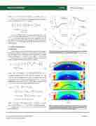
FIG. 5. Frequency and growth rate of the ITG mode dependence on k?qi in panels (a) and (b) and dependence on s 1⁄4 Te/Ti in panels (c) and (d).
FIG. 6. (a) Magnetic poloidal flux normalized by a separatrix value: w=jwOj, (b)–(d) are total magnetic field B, radial magnetic field BR, and axial magnetic field BZ nor- malized by B0 1⁄4 531 G. The circles represent the separatrix.
1⁄4 Te=mi is the ion sound speed. By applying the Fourier transform in the toroidal direction to Eq. (31), we have
e2n " Z2 e2 n T ! n # i0i2 e0i2 e0
􏰂 q 1þ
e2 s Zi2 ni0 Te
r ðnÞþ ?
dwðnÞ
ni0
Te0 1⁄4ZidniðnÞ
1
e2n T :
(32)
Z ni0 Te0 i
scitation.org/journal/php
where dw1⁄4d/􏰂 pffiffiffiffiffiffiffiffiffiffiffiffi
Ti0 Zini0
􏰍 e2 ne0 Ti0􏰎
dni= 1þ 2 ;qs 1⁄4Cs=Xci, and Cs
1þ e0 i0 Zi2 ni0 Te0
For each toroidally spectral component with mode number n, we carry out central finite difference of r2?ðnÞ as shown by Eqs. (15)–(17) on the (R, Z) plane and construct the tridiagonal matrix on field aligned simulation grids. Then, the sparse discrete matrix equa- tion for Eq. (32) is solved using the Krylov method implemented in PETSc software.
IV. CODE VERIFICATION A. Slab limit
In this section, we show the benchmark results of GTC-X against the analytical dispersion relation in an approximately uniform mag- netic field (ignore the ion diamagnetic and curvature drifts). Applying Fourier transform @t 1⁄4 􏰂ix; b0 􏰀 r 1⁄4 ikjj, and r? 1⁄4 ik? for Eq. (22) in linear plasmas in a uniform magnetic field, we can derive the linear perturbed distribution of gyrokinetic ion species
( " mv2þ2lB !#
1 Zi􏰈 ijj 0
dfi1⁄4 􏰂 xi 1þ x 􏰂 kjjvjj Ti
2Ti
􏰂1:5 gi
(33)
Zkv)
þ i jj jj hd/ifi0;
Ti
where hd/i 1⁄4 1 Þ d/ðxÞdf 1⁄4 P d/ðkÞexpðik 􏰀 RÞJ 􏰍k? v? 􏰎; x is
2p k 0 Xci
the particle position, and R is the gyrocenter position, x􏰈 1⁄4 cTi
􏰐 Z i n i 0 Z i n i 0 x 􏰂 x 􏰈i hdnii1⁄4 􏰂 􏰂 niZðniÞ
i ZiB0 1 @ni0 kf is the ion diamagnetic drift frequency (negative value for the
ni0 @r
normal profile which decreases along the R direction), kf 1⁄4 n=R is the perpendicular wave vector, and gi 1⁄4 dlnTi=dlnni0. Integrating Eq. (33) to the 0th order, the ion density perturbation becomes
Ti Ti x
􏰑 􏰁C 􏰂k2 q2􏰀d/þZini0 g x􏰈i nZðnÞ􏰁􏰂1􏰂k2 q2􏰀
Z i n i 0 x 􏰈i þ gi
x 􏰈i 2Ti x
2 3 Z i n i 0
ni 1⁄21 þ niZðniÞ􏰃􏰂 gi
niZðniÞ 0?i Tiixii ?i
Ti x
􏰁 C0􏰂k2?q2i 􏰀 þ k2?q2i C1􏰂k2?q2i 􏰀􏰈d/; (34) C0ðk2?q2i Þ 1⁄4 I0ðk2?q2i Þexpð􏰂k2?q2i Þ; C1ðk2?q2i Þ 1⁄4 I1ðk2?q2i Þ
where
expð􏰂k2 q2Þ and Zðn Þ 1⁄4 p􏰂1=2 Ðþ1 dtexpð􏰂t2Þ is the plasma function.
?i i 􏰂1 t􏰂ni
Combing Eqs. (34), (25), and (26), we can derive the linear dis-
persion relation as15
Phys. Plasmas 26, 042506 (2019); doi: 10.1063/1.5087079 Published under license by AIP Publishing
26, 042506-8
^