Page 2 - Demo

10E503-2
Roche et al.
Rev. Sci. Instrum. 83, 10E503 (2012)
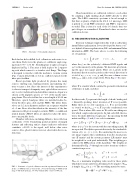
FIG.1. Schematicoftomographicdiagnostic.
Each fan has holes drilled for 8 collimators and screws to se- cure them. Each views the plasma at a different angle rang- ing from 37.79◦ to 71.04◦. Resulting line of sight coverage is displayed in Fig. 1. Fan array is held in place by 2 support- ing rods which connect to a stainless steel flange. The flange is designed to interface with the machine’s vacuum system (Fig. 1) and is fitted with a 2 3/4 in. conflat receptacle for the fiber optic feedthru.
Broad spectrum light produced by plasma has many sources: emitting ions, emitting neutrals, and radiating elec- trons to name a few. Since the interest of this experiment is to observe transport of impurity ions, optical filters are neces- sary to select radiation from desired line emission. Argon was chosen as the impurity species at ∼1% of the mostly nitro- gen plasma. The selected line has a wavelength of 434.8 nm. Therefore, optical band-pass filters are installed in-line be- tween the fiber optic cable and the PMTs. The filters them- selves are 1/2 in. in diameter and have an acceptance window of ∼1 nm. Even after this filtration the intensity of the line emission is still great enough to saturate PMTs, so additional neutral density (ND20) filters are added to reduce the inten- sity to measurable levels.
Chamber reflections, including diffusive, have reflection coefficients <0.04. Considering spatial geometry of imaged features and reflecting surface shapes indicates reflections contribute <0.01% to the signal, well below other noise sources. Also, ghost features were not observed in the recon- structions.
FIG. 2. Schematic of optical collimators used in experiment. Dimensions in inches. (1) SMA mount, (2) lens mount, (3) lens mount ring, (4) SMA mount ring, (5) Thorlabs LA1222, (6) 905 polymide fiber connector 600 μm.
Chord sensitivities are calibrated, relative to each other, by coupling a light emitting diode (LED) directly to fiber optic. The LED’s emissivity spectrum is broad enough so that there is plenty of light in the 434.8 ± 1 nm range. LED is pulsed (to avoid PMT saturation) and PMT’s response is recorded. This is done for each of the 16 chords, then out- put voltages are normalized. Normalized values are used as calibration factors.
III. RECONSTRUCTION ALGORITHM
Inversion technique employed in this work is called min- imum Fisher regularization. It was developed by Anton et al.7 as a hybrid of linear regularization (LR) and minimum Fisher information (MFI). The basic idea is to solve the following set of equations:
fl= dsg(r) l=1...nl, (1) Sl
where the fl are the (relatively) calibrated PMT signals and g(r) is the emissivity of the plasma. We discretize g by break- ing the space into square pixels. There are nx pixels in the horizontal direction and ny pixels in the vertical direction for a total of npixels = nx × ny. g and f become column vectors with npixels and nl rows, respectively. Then, Eq. (1) becomes
f = T ∗ g, (2) where T is a matrix which contains the geometric information
of the lines of sight, such that Tli =
In other words, Tli represents the length of chord l inside pixel i. Generally speaking, direct inversion of T is not possible. Either there are too few equations, i.e., T is not invertible or, even if we had npixels = nl, T is poorly conditioned (very sparse). This is where LR comes in. We add a smoothing ma- trix which couples adjacent pixels. In 2nd order LR, the ma- trix is the finite-difference Laplacian.7 Incorporating the LR matrix and Eqs. (2) and (3) we seek to minimize
φ= 1 (T˜ ∗g− ˜f)T ∗(T˜ ∗g− ˜f)+gT ∗H∗g, (4) 2
where φ is χ2 for the system with the smoothing matrix, H,
incorporated. The tildes represent division by the standard de-
viation of f , i.e., f˜ = f /σ . Reconstructing the most accu- llll
rate image requires that contributions from the chord geom- etry (T matrix) and the system geometry (LR matrix) must be weighted for each pixel individually. This weighting pro- cedure is the MFI portion of the algorithm.7 The weights are determined by Eq. (5) through successive iterations of the re- construction process.
(n)1(n−1) ·δij W(n)= 2gi gi
ij Wmax·δij
Wmax is a maximum weighting value used for those pixels which have erroneously been determined to be negative. Wmax is simply 1/gmin for gi > 0. The smoothing matrix becomes,
(n) T (n)
H→H = ∗W ∗ , (6)
Sli
ds. (3)
g(n) >0 n>0
i (5)
g(n)≤0 n>0 i