Page 6 - Feasibility study of microwave electron heating on the C-2 field-reversed configuration device

012509-6
Fulton et al.
Phys. Plasmas 23, 012509 (2016)
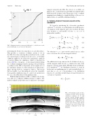
FIG. 1. Mapping from the geometry poloidal angle, h, to the Boozer coordi- nate poloidal angle, hB on a reference flux surface.
performing the Fourier decomposition on each flux surface. This provides a consistent coordinate system to use in the SOL. Note that enforcing this periodicity for the coordi- nate transformation is distinct from the choice of boundary conditions applied to the field solver and particle equations of motion during the simulation, which is discussed in Section III. One consequence of enforcing periodicity during the coordinate mapping is that the spacing of the poloidal hB -coordinate in the SOL is dependent on the length, in Z, of the simulation domain. A wider domain in Z will produce larger spacing between constant-hB surfaces. This means that necessarily, hB is discontinuous across the separatrix. Consequently, simulations may be carried out separately in the core or the SOL but not both simultaneously.
With this implementation of SOL coordinates, the descrip- tion of Boozer coordinates in FRC geometry is complete. The method outlined in this subsection is sufficient to investigate
0
v_1⁄4 0 ðl$BþZ$/Þ a
transport isolated in the SOL. The effects of core-SOL cou- pling are also of critical interest and will be investigated with a different model in future work. Progression of the coordinate mapping from cylindrical to straight field line to Boozer coor- dinates in the core and SOL is illustrated in Fig. 2.
III. FORMULATION OF POISSON SOLVER IN FRC GEOMETRY
We begin by introducing the electrostatic gyrokinetic equations58 to describe a toroidal plasma in an inhomogene- ous magnetic field, using the gyrocenter position, X, mag- netic moment, l, and parallel velocity, vk, as a set of independent variables
df X;l;v;t "@þX_ $þv_ @ C#f; (14) dta k @t k@vkaa
X_ 1⁄4 v B0 þ v þ v ; kBEd
(15) : (16)
The subscript, a 1⁄4 e; i, represents the particle species, either ions or electrons. The effective magnetic field is
B 0 1⁄4 B0 þ B0vk r b0: (17) Xa
The additional velocity terms are the E B drift velocity, vE, and the magnetic drift velocity, vd, which is the sum of the magnetic curvature drift and the $B drift. In the perturbative ðd f Þ simulation,59–62 the distribution function, fa, may be broken into an equilibrium part, f0, and a perturbed part, d f , such that fa 1⁄4 f0 þ d f . Corresponding to the distribution function, we can define perturbed gyroaveraged densities for each species of particle
ð
dna 1⁄4 dfad3v: (18)
FIG. 2. Poloidal plane meshes for three coordinates systems. In the top panel, cylindrical coordinates, (R, Z), with contours beneath showing magnetic flux extracted from the LR_eqMI input equilibrium. In the middle panel, the straight field line coordinate mesh, ðwf;hfÞ. In the bottom panel, Boozer coordinates, ðwB;hBÞ are shown. The separatrix is indicated by the wide black line.
1 B
k mB 0 a mc@t
Z @Ak a0a