Page 3 - A combined mmwave and CO2 interferometer on the C-2W Jet plasma

Nucl. Fusion 58 (2018) 082011 2.5
2.0
1.5
1.0
0.5
0.0
2.2 2.3
R.M. Magee et al
mode energy (a.u.)
f (kHz)
mode frequency (MHz)
tonset (ms)
2.4 2.5
Bext ne-1/2 (104 G cm3/2)
2.7
2.8 2.9
0 02468
tcritical (ms)
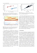
Figure 5. Mode onset. tcritical is defined as the time at which
ρfi = 1.3rs. As illustrated above, this is found to be approximately equal to the onset time for fluctuations.
We noted above that this mode appears only late in the dis- charge. As a final characterizing observation, we can roughly quantify the onset time as a function of the fast ion gyro radius and the separatrix radius. The fast ion gyro radius is calculated using ρfi = vfi/ωci, where vfi is the velocity of the fast ions at the injection energy and ωci is the cyclotron frequency calcu- lated in the open field line plasma. The separatrix radius, rs, is defined as it is in the tokamak, as the boundary between closed and open field lines. Empirically, we find that the onset time for fluctuations, tonset occurs when ρfi ≈ 1.3rs. In figure 5 this time is defined as tcritical and plotted against tonset to illus- trate the quality of the linear relation.
Early in the discharge, when ρfi < rs, most fast ions do not execute complete gyro orbits, but instead execute beta- tron orbits, dipping in and out of the FRC as they circle the device. Late in the discharge, when ρfi > rs, most fast ions can execute complete gyro orbits. The appearance of the mode is likely related to this change in orbit topology.
4. Interpretation
For a subset of C-2U discharges, the radial density profile has been reconstructed using Abel inverted FIR data in conjunction with edge Langmuir probe measurements. With an accurate density profile, it is possible to reconstruct the radial profile of the m = 0 compressional Alfvén continuum, defined as
fA = nvA/(2πr) where n is the azimuthal mode number, VA is the local Alfvén velocity, and r is the plasma radius. We use an idealized rigid rotor model for the magnetic field profile [14] in which the magnetic field strength varies weakly with radius outside of the separatrix, dropping only 15% from the wall at r = 70 cm to r = 40 cm, so the variation in the Alfvén velocity is largely due to changes in density in the open field line plasma.
Shown in the bottom frame of figure 6 are fA(r) profiles for three different time windows, corresponding to the times of Alfvén mode activity. For example, as seen in the top frame of figure 6, the n=4 mode is active from t=5–7ms. The average fA(r) profile over that time window is plotted as the solid curve in the bottom frame. The average observed fre- quency (again, as given by the spectrogram) is 1.75 MHz. This frequency on the outboard side of the fA(r) profile occurs at
Figure 3. Mode frequency scaling. The lab frame mode frequency is proportional to the measured edge Alfvén velocity. Higher frequency modes (red) are typically n = 4; lower frequency modes (blue) are typically n = 3.
2000 1500 1000
500
0
5
n=1
n=2
4 n=3
3 2
1
0
5 6 7 t (ms) 8 9 10
Figure 4. Time resolved n-spectra. The top frame shows the edge Mirnov probe magnetic spectrogram and the bottom frame the corresponding SVD traces. Alfvén modes typically have n = 3, though n = 4 and n = 2 are also observed.
The azimuthal array (see ‘NB plane array’ in figure 1(b)) is composed of 8 magnetic pick-up coils. By calculating the fast Fourier transform (FFT) of the time series of each probe signal and comparing the coil-to-coil phase around the array, one can determine the azimuthal or toroidal mode number, n and the direction of propagation, which turns out to be co- propagating with the injected beam ions.
In order to investigate the temporal dynamics of the modes, it is more efficient to use singular value decomposition (SVD) analysis [13] than the FFT. This is a standard technique in which the time series data from the probes are cast as a matrix, with each column a single probe and each row a single time point. The eigenvalues of the matrix give the normal modes, which are shown as functions of time in figure 4.
It is interesting to note the cyclic behavior of the chirping n = 2 mode and the n = 3 Alfvén mode. Large amplitude n = 3 mode is sustained for 200–300 μs and then interrupted by short-lived bursts of n = 2 mode. The n = 3 reappears only after the n = 2 has died down. Sometimes a higher frequency n=4 mode crops up just after the demise of the n=2 and just before the emergence of the n = 3 (see figure 4, bottom frame just before and just after t = 6 ms).
2.6
n=4
3
8 6
4
2