Page 13 - Theory of ion dynamics and heating by magnetic pumping in FRC plasma

072510-13 Egedal et al.
Fj1⁄4 A􏰊j;0Cj;j @fs:
Phys. Plasmas 25, 072510 (2018) B􏰊0;j ’ 1 @A􏰊0;jvJ0 : (35)
vJ0 @v
Equation (35) can then be used as a check on the applicabil-
ity of the approximations introduced with Eq. (34). B. Numerical example for parallel compression
For both the full model and the reduced model in Eq.
(34), there are no couplings between different values of p/.
This is because p/ is a true constant of motion during the
pumping process, and the rate of ion heating by MP can
therefore be examined separately for any particular value of
p/. As an example, we apply Eq. (34) to the case p/ 1⁄4 p/0,
with qW0 1⁄4 p/0 corresponding to the flux surface
highlighted in blue in Fig. 1 (thus, points along orbits for
which v/ 1⁄4 0 lie on the highlighted W 1⁄4 W0 contour). This
value of p/ was also applied to compute the profiles in Figs.
9(d)–9(f) and 12. In turn, the function D/B in Eq. (17) as
well as Tk;j; A􏰊k;j, and B􏰊k;j in Eq. (26) are then easily evalu-
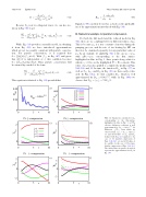
ated. In Fig. 14(a), we first consider D/B, which is well
(32) Because Tk;j now is a diagonal tensor, we can also iso-
late f0s in Eq. (30) to get
@f0s x2 X􏰏􏰊 @ 􏰊 􏰉
0;0 j
1⁄4 0: (33)
@t þ 2T
A0;j @v Fj þ B0;j Fj
x 2 T 02 ; 0 þ C 2j ; j @ v 0
While Eq. (33) provides a tractable model, in obtaining it from Eq. (30) we have introduced approximations which are not necessarily consistent with particle conserva- tion.Ð For particle conservation, it is required that 0 1⁄4 ð@f0s@tÞ J v;n dv dn. With J v;n in Eq. (A7) and given that Ð@f0s=@t is independent of n, this condition becomes 0 1⁄4 T0;0 vJ0 ð@f0s=@tÞ dv. Thus, particle conservation will be ensured by a model of the form
(34)
s2X
@f0þ x @A􏰊0;jvJ0Fj1⁄40:
@t 2T0;0vJ0 j @v
This equation is identical to Eq. (33) provided that
approximated by D/ ’ 0:06=v0:8, while in Fig. 14(b) we B pffiffi
observe that T0;0 1⁄4 hsbin 1⁄4 720= v.
FIG. 14. Parameters calculated for p/
corresponding to the flux-surface
highlighted in blue in Fig. 1. (a) The
effective diffusion coefficient is well
approximated by D/ ’ 0:06=v0:8. (b)
pffiffi B
Functions v T0;j , from which we
pffiffi observed that hsbin 1⁄4 T0;0 ’ 720= v.
(c) and (d) Profiles of A􏰊0;j and B􏰊0;j defined with Eq. (26) applied to the case of 1% parallel compression of Figs. 9(d)–9(f). (e) and (f) Profiles of A􏰊0;j and B􏰊0;j for the case of 1% perpen- dicular compression of Figs. 9(a)–9(c). The dashed lines in panels (d) and (f) represent the approximation for B􏰊0;j in Eq. (35).