
Page 1 - An Interesting Poster to look at from the Tri Alpha Energy Team in California
P. 1
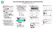
Reconstructing FRC equilibria from experimental data
Loren Steinhauer, Thomas Roche, Joshua Steinhauer,
TAE Technologies, Inc., 19631 Pauling, Foothill Ranch, CA 92610
PREVIEW of “Grushenka”
The magnetic structure of FRCs cannot be measured directly by existing diagnostics. A new tool “Grushenka” finds the structure based on magnetic measurements at the vessel wall. The ingredients are
Data conditioning, finding smooth fits to two sets of data --excluded flux radius, R(z)
--wall magnetic flux, w(z)
Distill scalar values, three each from the excluded flux
and wall flux profiles.
Equilibrium finder: model - static equilibrium (Grad-
Shafranov = “GS” equation). Inputs to GS system p() function and w(z).
--employ a three parameter form of the pressure function p = p(;C1, C2, C3)
Nested iterative solver
--successive over-relaxation solver for (r,z)
--iterative procedure to adjust parameters (C1, C2, C3). The iteration proceeds until (a) (r,z) is consistent with
the GS equation and (b) it replicates measurements.
Post-processing: yields a host of quantities that cannot be measured. For example
--actual FRC core dimensions: Rs, Zs
--trapped magnetic flux p
--plasma current in core IC and periphery IP --plasma inventory in core NC and periphery NP --stability indices: tilt, tearing, interchange
PRACTICAL ATTRIBUTES OF Grushenka
Essentially instantaneous computation. Using a coarse 2D grid, computation of a whole-shot sequence of equilibria takes ~10 seconds on an ordinary PC.
--Grushenka useful for control room “between- shot” scrutiny of critical performance parameters
No presumption of a transport model, i.e. guesswork about the transport model. It only depends on the validity of an evolving quasi-equilibrium (QeQ).
--QeQ allows Grushenka to track straight through relaxation events, which is impossible for a 2D transport model. (FRCs are widely believed to be relaxing objects.)
APPROXIMATIONS IN Grushenka PHYSICS MODEL
Static plasma p = j B (evolving quasi-equilibrium)
--QeQ a good assumption in TAE experiments because the dynamical timescale (<10s) is much smaller than experiment lifetimes (several ms)
Flexible pressure function p = p(;C1, C2, C3) --Three-parameter flexibility allows access to most
features of practical pressure profiles (see figure) C1 : magnitude of pressure – mostly affects Rs
C2 : core pressure and current – mostly affects Zs
RECONSTRUCTION EXAMPLE: C-2W #107,251
Flux contours (r,z) = const at t = 0.5ms
Mid-plane radial profiles - early and mid-life times: flux , pressure p, magnetic field Bz, current density j/r
Evolution of core and periphery contributions to inventory and current
** Core contributions are only about 1/3 of the total. Dashed lines on inventory are exponential fits with decay time N = 4.8ms
Evolution of stability indices
> Tilt stable if S*/E < ~2.5 S* = Rs/i
(i = ion skin depth) elongation E = Zs/Rs
Interchange and tearing: positive index stable
Interchange unstable late; tearing stable except possibly very early
ENHANCEMENTS IN PROGRESS (“Hyperion” tool)
Fully-kinetic treatment of ions
Fluid-electron model
Edge biasing
Thermal and super-thermal ion components
Stay tuned.
C
: edge gradient – mostly affects L
(SOL thickness)
3
p
peaked current C2 < 0
hollow current C2 > 0
j/r = p() Current
magnitude C1
thin SOL large C3
t = 0.5ms Early
t = 3ms mid-life
thick SOL small C3
/R
Mathematical construct: Grad-Shafranov equation
* = 0r2p() + Boundary conditions Computational domain: figure relevant to C-2W facility
Time histories: dashed lines = measured; symbols = reconstructed
Evolution of radial and axial dimensions of FRC radii: R = excluded flux, R = separatrix
s
half-lengths: Z2/3 = excluded flux, Zs = separatrix
B.C. = w(z)
r Rwall = 0.8m
End cone
/n = 0 z
Zmax
=2.9m
/n = 0
Zmax
= 0
0
Metal wall
axis
EXPERIMENTAL INPUTs
Symmetry plane
** C-2W: excluded flux values good approximations; C-2U (not shown) shows differences: shorter plasmas so that Rs can exceed R
Evolution of trapped flux p “Rigid-rotor” approx.
RR = BeR3/Rwall
Be = wall radius at mid-plane
** C-2W: RR formula fairly good except at early times; C-2U: p exceeds RR by factor of 1.5 at late times
(at each time instant) wall flux profile w vs z
excluded flux radius (mid-plane) R0
excluded flux half-length Z2/3
(future) edge thickness (gradient length)
| 1 |
