An Interesting Poster to look at from the Tri Alpha Energy Team in California

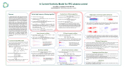
A Current-Vorticity Model for FRC plasma control
S. A. Galkin, J. A. Romero and the TAE Team
TAE Technologies, Inc., 19631 Pauling, Foothill Ranch, CA 92610
Abstract
A current-vorticity MHD model and code have been developed for FRC plasma control applications in the C-2W device [1]. The model uses a flexible filtering technique to restrict the frequency bandwidth of the simulations to the control bandwidth of interest. For dynamic systems written in the state space form 𝑥ሶ = 𝐹 𝑥, 𝑡 + 𝑈(𝑡), we propose an algorithm based on a frequency domain eingenvalue analysis to remove frequency components above a certain frequency threshold of interest, typically determined by the desired control bandwidth. For small systems of a few states this filtering technique works effectively. For systems with a large number of states, a direct calculation of the Jacobian and its eigenvalues becomes impracticable, so we have developed a modified method which reduces the number of states (shrinking to a small system), filters and reconstructs the original high order system using a Gaussian Process inversion technique. The main purpose of the plasma model is to be applied to control system design, whose function is to maintain macroscopic plasma parameters such as shape, position, elongation, etc. at prescribed values. Details of the model and simulations will be presented.
A current-vorticity MHD model
◼ The 2D non-linear dynamic integral-differential reduced MHD model written in the state space form 𝑥ሶ = 𝐹 𝑥, 𝑡 + 𝑈(𝑡) for plasma control application includes:
◼ four differential governing equations: for the plasma current density 𝑗 , for vorticity ω, for induced currents in
magnets/wall Iext and for mass density ρ: 𝜇𝜕𝑗𝜑=−∆ (𝒗×𝑩)−𝜂𝑗
Active high frequency filtering algorithm
Practical form of filtering algorithm
We can find a linear operator C, which provides such behavior near x0:
Single plasma current loop inside C-2W device
Magnetic system of C-2W (magnets and conducting CV) was used for simulation of one single plasma loop dynamics
◼
◼ Linearization of the non-linear operator F(x) near x0 can be done with
◼ ◼ ◼ ◼ ◼
෩
𝐶𝐹𝑥 =𝐽𝑥+𝑅(𝑥)
◼
Consider non-linear dynamic system
00
𝑥ሶ = 𝐹(𝑥)
𝐹 𝑥 ≈𝐹 𝑥0 +𝐽(𝑥0)(𝑥−𝑥0)
Substituting F from the Taylor expansion, with some algebra we get:
Jacobian operator J(x0)
◼ The Jacobian matrix can be presented through a diagonal matrix Λ of its
Therefore we have the modified filtered dynamic system:
෩ −1 𝑥ሶ=𝐶𝐹𝑥=𝐽𝐽 𝐹(𝑥)
eigenvalues and left eigenfunction matrix U as 𝐽 =𝑈−1Λ𝑈
◼ use a threshold ωcrit to separate low frequency spectrum from
undesirable high end of the oscillating spectrum. It can be done for all
෩ 00◼
There are higher frequency oscillations of r(t) and lower frequency in z(t). Plasma current and induced eddy currents in the CV contain high frequency oscillations. Simulation with I (0)=0.3MA, for r(t),
0
The filtering algorithm for the original non-linear dynamic system consist of finding the Jacobian J and the filtered Jacobian, defined by
p z(t), Ip(t) and Icv(t) - all red curves, blue – filtered with ωcrit =5kHz threshold.
not growing eigenvalues with Re(Λ)≤0 and |Im(Λ)|> ωcrit by replacing ෩
until t0+ΔT, after that both Jacobians should be recomputed and solution is continued. Value of ΔT depends on properties of the original system and might vary from a few time steps to many time steps.
2D linear harmonic oscillator
Consider 2D linear harmonic oscillator with coordinates x(t), y(t) and velocity vx(t), vy(t), with coefficients k:
𝑚𝑣ሶ =−𝑘 𝑥−𝑘 𝑦−𝑘 𝑣 𝑥 𝑥𝑥 𝑥𝑦 𝑥𝑣𝑥
𝑚𝑣ሶ =−𝑘 𝑦−𝑘 𝑥−𝑘 𝑣 𝑦 𝑦𝑦 𝑦𝑥 𝑦𝑣𝑦
The system has “low” and “high” frequency spectrum if we choice kxx>>kyy. Filter with ωcrit ≈0.5(ωlow +ωhigh) suppresses high frequency oscillations with dumping and reproduces low frequency oscillations.
Figure. Results with kxx/kyy=100. Original (red) and filtered (blue) solutions. Both original and filtered y(t) coincides (bottom plot)
2D non-linear harmonic oscillator
𝐶=𝐽𝐽 00
෩ −1
The system can be solved in two steps:
𝐽 𝑢 = 𝐹 𝑥 , 𝑥ሶ = 𝐽 𝑢 (*)
0
ωcrit, then solution to the system (*). Such filtered solution will be valid
00
their imaginary parts with 0. Therefore we get filtered Λ and can reconstruct a filtered Jacobian
෩ −1෩
𝐽 =𝑈 Λ𝑈
0
◼ Desired filtered behavior of the system near x0 is then governed by:
෩
𝑥ሶ = 𝐽 𝑥 + 𝑅(𝑥 )
00
Linear harmonic oscillator
◼ Linear harmonic oscillator, which has analytic solution, is a good starting test for the filtering algorithm:
◼
◼
◼
Fast oscillations were completely suppressed, slow spectrum dynamics was resolved. Accuracy: see the original and the filtered z(t) on the same plot. Amplitude and phase of the filtered solution slightly diverge in time, but many period were computed and time interval ΔT for Jacobian refreshing was pretty large: ΔT=100dt, dt - time stepping.
Filtering of large system
◼
𝑥ሷ + 2𝜉𝜔 𝑥ሶ + 𝜔2𝑥 = 0 00
Analytic solution contains one frequency and dumping. In this case we cannot separate “low” and “high” frequencies but we can suppress oscillating solution to critical dumping solution:
Figure. Analytic solution was reproduced numerically (red curve) and critical dumping was computed with the filtering algorithm (blue curve)
Non-linear oscillator
Non-linear 1D oscillator (an analytic solution maybe unknown):
𝑥ሷ + 2𝜉𝜔 𝑥ሶ + 𝜔2𝑥3 = 0 0 0
We expect to see “critical dumping” if the filtering is applied. computed solution (red curves) exposes more complex behavior then linear oscillator. Computed filtered solution (blue curves) can be considered as “dumped” solution to non-linear oscillator.
Figure.Computedoriginal(red curves) and filtered (dumped – blue curves) solutions to non-linear oscillator
𝜑
◼ For large system (hundreds of thousand equations) computing of Jacobian becomes impractical. Large system can be clustered to a small system of cluster equations, which can be filtered effectively.
◼ Clustering can be done with a linear projector operator P acting on large vector-column {x}N of size N and transferring it into much smaller vector {y}K , K<<N: 𝑦 = 𝑃𝑥.
◼ We apply the filter to small cluster system with Jacobian j0 and then reconstruct filtered solution to the
original system either with Moore–Penrose inverse (or pseudoinverse, P+) or Gaussian exponential
covariance pseudoinverse [2] (or g-pseudoinverse, P +): g
ሶ +෩−1 𝑥෤=𝑃(𝑗0𝑗0 𝑃𝐹(𝑥))
Ongoing work and future plans
◼ For current-vorticity model in integral-differential form, the Jacobean can be computed analytically. This was done and the analytic Jacobian is under testing now.
◼ Choice of clustering projector operator P as well as Gaussian exponential covariance pseudoinverse P +
can be optimized for better accuracy. This is ongoing and future plan.
◼ Accuracy of the filtering algorithm can be further improved with Gaussian matrix inversion also.
◼ The filtered current-vorticity model will be incorporated into plasma control system of C-2W and future
machine.
References
◼ [1] H. Gota et al., Nucl. Fusion 59, 112009 (2019).
◼ [2] J. Romero et al. Inference of field reversed configuration topology and dynamics during Alfvenic
transients. Nature communications 9, 691 (2018)
0𝜕𝑡 𝜑 𝜑 𝜑
𝜕𝜔 𝑣𝜔𝜕 𝜕 =−𝒗∙𝛻𝜔+ 𝑟 + 𝐵𝑗/𝜌+ 𝐵𝑗/𝜌
𝜕𝑡 𝑟 𝜕𝑟𝑟 𝜕𝑧𝑧
𝑀𝑑𝐼𝑒𝑥𝑡=−𝑅𝐼 −𝑀𝑇 𝜕𝐼+𝑈 𝜕𝜌 𝑑𝑡 𝑒𝑥𝑡 𝑒𝑥𝑡 𝜕𝑡 𝑒𝑥𝑡
𝜕𝑡 = −𝒗 ∙ 𝛻𝜌
◼ integral (matrix) equations for the magnetic flux and field: 𝜓=𝑀𝐼+𝑀 𝐼
◼ ◼
◼
◼
2D non-linear harmonic oscillator with coordinates x(t), y(t) and velocity v (t), v (t), with coefficients k:
𝐵 = 𝑃 𝐼 + 𝑃 𝐼
𝑟 𝑟 𝑒𝑥𝑡𝑟 𝑒𝑥𝑡
𝐵=𝑃𝐼+𝑃 𝐼
𝑧 𝑧 𝑒𝑥𝑡𝑧 𝑒𝑥𝑡
◼ integral (matrix) equations for plasma velocity: 𝑣 =𝑈𝜔
g
𝑝 𝑒𝑥𝑡 𝑒𝑥𝑡
𝑚𝑣ሶ =−𝑘 𝑦 −𝑘 𝑦𝑥−𝑘 𝑣 𝑦 𝑦𝑦 𝑦𝑥 𝑦𝑣𝑦
xy3
𝑚𝑣ሶ =−𝑘 𝑥 −𝑘 𝑥𝑦−𝑘 𝑣
𝑥 𝑥𝑥 𝑥𝑦 𝑥𝑣𝑥
3
“Low” and “high” frequency spectrum exist if we consider large enough ratio of coefficients. For the simulations below kxx/kyy=104 was used.
Figure. Unfiltered solution x(t), y(t), vx(t), vy(t) – all reds; filtered solution – all blues, filtering was applied after 5 sec.
𝑟𝒓
𝑣 = 𝑈 𝜔 𝑧𝒛
◼ Proper
integral form, initial conditions complete the model.
into the
boundary conditions
have been
included