Page 3 - Detection and prediction of a beam-driven mode in field-reversed configuration plasma with recurrent neural networks

Nucl. Fusion 60 (2020) 126025 C. Scott et al
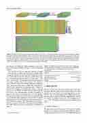
Figure 2. Illustration of data preprocessing pipeline. Windows of 0.2 ms are extracted from shots, centered so that all instrument readings have unit normal mean and standard deviation, and then converted into principal components. Top: illustration of entire process, with each ‘window’ rendered as a 2D array. Center: One ‘raw’ window e.g. prior to normalizing and PCA. Bottom: One window post-processing. In each 2D representation, columns represent input probes, and rows represent successive timesteps (from top to bottom). Plots of several of these probe readings as a function of time (for one shot) may be found in figure 3. Normalizing, followed by PCA, reduces the numerical spread of the input values as well as reducing the dimensionality of the input.
the efficiency of training the ANN and improve the perform- ance of the mode prediction. See figure 7 and accompanying caption.
For each shot, we slice the input into ‘windows’ of length 0.2 ms, and take a random selection of these windows. Each is tagged as staircase or non-staircase depending on the output of a Canny edge detector [9] on the R∆φ signal. Canny edge detection marks locations in a signal as ‘strong edge’, ‘weak edge’ and ‘no edge’. We interpret the first two as instances of staircase, and the latter as non-staircase. The dataset is then a 3D stack of these 2D windows, with axes correspond- ing to data index, probe index, and time. We normalize over both the time and probe axes simultaneously, so that for a given probe, readings over all times have mean μ = 0.0 and std. dev. σ = 1.0. Finally, we apply principal component ana- lysis (PCA) [10], with whitening, to reduce the number of inputs to the neural network from 360 to 270. This pipeline was built using scikit-learn [11], the data was randomly4split into a training set and a validation set at a ratio of 85-15, and all transforms were fit to training data and then run on validation data (without re-training). All of the models in the next sec- tion were created in Tensorflow [12] and run on an NVIDIA k20 GPU. This data preprocessing pipeline is illustrated in figure 2.
4 With a fixed random seed.
Table1. Comparisonofmethodssurveyedinsection3(staircase classification task). Among the several models tested, LSTMs had the best performance at classifying shots as staircase or non-staircase.
Method
Convolution (separate towers) Convolution (joined)
RNN (one hidden layer) LSTMs
3. Model selection
Accuracy (% correct)
64.5 Did not converge 75.0 84.7
3
We next evaluate several neural-network models on this clas- sification task. For each network detailed below, the final network layer was a binary vector encoding staircase or non- staircase. We used mean-squared error (MSE) between tar- gets and outputs, minimized with the AdamOptimizer (which is a variant of gradient descent [13], with learning rate set to 1 × 104 ). All models detailed below are summarized in table 1.
3.1. Model architecture
We first provide a short description of the machine learning models used. Artificial neural networks (ANNs) are univer- sal function approximators: there are well-founded theoretical