Page 5 - Detection and prediction of a beam-driven mode in field-reversed configuration plasma with recurrent neural networks

Nucl. Fusion 60 (2020) 126025 C. Scott et al
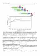
Figure 4. Top: structural schematic of most accurate LSTM model. Each green rectangle represents one output of the data preprocessing pipeline, as in figure 2. Red bars within each rectangle indicate which timestep is being fed into the LSTM. Each blue box labeled ‘LSTM’ represents the same neural network; for each time step in a given sequence of data the LSTM takes as input one timestep and the previous hidden state, and outputs the next hidden state. Bottom: Typical training run of same model. Accuracy of staircase prediction is plotted as a function of number of training batches, both for the training data batch (blue curve) as well as the held-out test dataset (red curve). The model learns to predict cases in the training data with 100% accuracy, but is less accurate on the test data, which it has not seen. .
image filter), rather than wasting computational effort compar- ing pixels which are far apart in the image. Typically, CNNs consist of a stack of ‘convolutional’ layers interspersed with spatial pooling, followed by several flattened layers which aggregate information from the entire (filtered, downsampled) image to make a final output prediction.
Another way for real-world data to be structured is to have an axis of the input data representing the same values over time. Recurrent neural networks (RNNs) process data by ini- tializing a random hidden layer as an initial internal state, and then stepping through a sequence of timesteps, after each of which the hidden layer is updated. Once the entire sequence has been processed, the value of the hidden layer is a latent rep- resentation of the sequence. Typically, the target output used to train RNNs is the next sequence element, i.e. predicting xt + 1 from some number of previous timesteps xt−k,xt−k+1,...xt. Various types of Recurrent neural network exist and detailing the differences is out of scope for this paper. These differences
are mainly in how the networks process sequences and how the new input and previous hidden state are combined to get the new hidden state. We use a variant called a long short-term memory (LSTM) network [21], which is distinguished by an internal subnetwork which uses logic gates to maintain a long term hidden vector representing the entire sequence, as well as a hidden vector representing local (in time) fluctuations.
3.2. Model development
In this subsection we detail early versions of the model, and the performance of each. We also discuss how these mod- els influenced design choices for the model described in section 3.3.
3.2.1. Convolution of individual diagnostics. For our first model, we applied separate convolutional network layers to
5