Page 5 - Demo

042504-5 Rath et al. Mathematically, Q2D uses
• One continuity equation for the ion and one for the neutral fluid.
• A momentum equation for each fluid.
• Ohm’s law for the electrons (to determine the electric
field).
• An energy equation for each fluid (to determine the
pressure).
• A heat flux proportional to the divergence of the tempera-
ture (using separate parallel and perpendicular thermal conductivities) to close the system.
The computation of the fluid magnetic field uses a boundary integral method, in which currents external to the plasma are represented by a distribution along segments that discretize the external coils and wall elements. The current density (per unit length) is assumed piecewise uniform per segment. This boundary integral description is combined with a uniform r,z mesh which describes the plasma domain. This is done with a cut-cell formalism that uses a uniform stencil for points that are strictly interior, ignores points that are strictly exterior, and applies a special difference stencil for points that are near the boundary of the domain.
The fluid momentum equations are solved using a semi- implicit method to avoid the CFL limit associated with wave propagation, and so very low density regions are allowed. The advective terms in the momentum equations are com- puted using the SMART algorithm.31
For the kinetic computation, the 2D magnetic and elec- tric fields and thermal background plasma profiles are imported from the fluid computation at each timestep. “New” fast neutrals that are injected with neutral beams are Monte Carlo sampled using calibrated parameters for focal length and divergence. Particle energy is distributed in the three components typical of positive ion neutral beam sour- ces. From this point on, fast neutrals are tracked kinetically. The trapping cross section in the background plasma is com- puted from standard formulae.32–34 When a fast neutral is trapped to become a fast ion, the kinetic fast ion orbit is advanced using the Boris push.35 Fast ion slowing and scat- tering on the background plasma (energy and heat exchange) are computed using the Monte Carlo method of Sherlock36 where the Fokker-Plank friction and diffusion coefficients are expressed in terms of a Langevin equation. When fast ions slow down below a certain threshold, they are absorbed into the background thermal plasma. Fast ions may charge exchange back to neutrals, at which point they are tracked
Phys. Plasmas 24, 042504 (2017)
and may be lost or may trap again as ions. When any colli- sion between a fast ion and the background thermal plasma or neutral population is computed, the result is accumulated in the Monte Carlo code by performing Particle In Cell (PIC) deposition using quadratic spline shaped particles. The results are applied as source and sink terms of the fluid energy, momentum, and particle density.
B. Initial conditions and unperturbed evolution
Both linear and non-linear simulations have been started from the same initial conditions. These conditions were obtained by starting with an arbitrary MHD equilibrium and letting the (non-linear) simulation run until a steady-state was achieved. The equilibrium magnetic field was in the order of 60 mT with a mirror ratio of 3.3.
Non-linear simulations were performed with the Q2D code. Linear simulations were run in Simulink, using the lin- ear system model computed with the modified VALEN code.
Current drive, fueling, and heating are provided by 6 neutral beams injecting 7 MW of 15 keV particles. In experiments, long-lived FRCs are additionally fueled by the cryogenic pellet or compact toroid injection. Either of those causes transient, large perturbations of the plasma equilibrium and thereby turns the coefficient matrices of the linear system into time-varying quantities. To avoid this complication, neither cryogenic pellets nor compact toroids were used in simulations for this work. Instead, fueling was provided by a hypothetical particle source inside the sepa- ratrix that provided a continuous stream of 1019 neutrals per millisecond.
In order to prevent the plasma from becoming axially unstable, all unperturbed simulations were run with super- conducting walls.
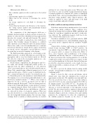
Figure 1 shows the flux contours and plasma current density after 1ms when the simulation has reached an approximate steady state. The simulation was run until 6 ms. Over the period from 1ms to 6ms, the separatrix radius is about ð37:560:5Þ cm, the separatrix length ð1:5060:05Þ m, the number density (3.2560.05) 1910 m 3, the plasma cur- rent ð16065Þ kA, and the total temperature ð260610Þ eV. The ratio of electron temperature to ion temperature is about 60:200. The take-away from these numbers is that the global plasma parameters are relatively constant throughout the simulation. Figure 2 shows the evolution of the axial stability parameter (Fzc in Equation (1)). Since the computation of the stability parameter depends on the choice of rigid
FIG. 1. Flux contours (blue lines) and toroidal current density (blue shading) at t 1⁄4 1 ms. The separatrix is highlighted in red. The green lines indicate some potential reasonable choices for the rigid volume: A spheroid that just barely encloses the separatrix, a cylinder of similar dimensions, or a spheroid that enclo- ses the majority of the plasma current. Black segments at the top indicate the position of control coils.