Page 6 - Demo

042504-6
Rath et al.
Phys. Plasmas 24, 042504 (2017)
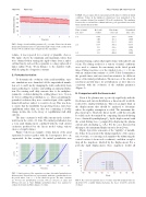
FIG. 2. Range of axial stability parameter Fzc over time. Plotted are the min- imum and maximum values for spheroidal rigid volumes with a radius from 42 cm to 70 cm (and the same elongation as the separatrix).
volume, it was repeated for a variety of plausible choices. The figure shows the minimum and maximum values that were obtained when varying the rigid volume from a spher- oid that barely enclosed the separatrix to a large spheroid of minor radius 70cm (10cm distance to the chamber wall), while keeping the elongation constant.
C. Perturbed evolution
To determine the evolution of the axial instability, sepa- rate simulations were branched off the unperturbed simula- tion at 1, 2, and 3 ms by changing the wall conductivity from superconducting to resistive and adding an initial perturba- tion. Pre-existing wall eddy currents (due to the midplane- symmetric evolution during the settling phase) were “frozen in” before adding the perturbation, i.e., when calculating the perturbed evolution, they were considered part of the equilib- rium field and not subject to resistive decay. This was done to ensure that the instability was growing from a static base equilibrium rather than one that was continuing to slowly change in time due to the decay of (equilibrium) wall eddy currents.
The time constant for wall eddy currents in the resistive wall was in the order of 1.2 ms. The initial perturbation was a 1cm axial displacement combined with the wall current excitation predicted by the linear model (using various choices of rigid volume).
Figure 3 shows an example of time history of the axial separatrix location together with the least-squares fit to an exponential. In this example, the initial perturbation was
Time of initial pert. (ms)
1.0
2.0
Rel. wall conduct.
0.50 1.00 1.50 0.75 1.0 1.75
Fitted time const. (ls)
193.9 383.1 556.7 307.4 394.6 671.8 400.4
Normalized time const.
0.506 1.000 1.453 0.779 1.000 1.702 1.000
FIG. 3. Axial position of the separatrix over time after initial perturbation at different times. Dotted lines are exponentials, with time constants fitted over the period where 2 cm < z < 12 cm (shaded in green). The time constants are 383.1 ls (for perturbations at 1 ms), 394.6 ls (for pert. at 2 ms), and 400.4 ls (for pert. at 3 ms). Multiple perturbation times were analyzed to estimate how much stability changes over time.
FIG. 4. Re-centered separatrix traces over time (run with nominal wall con- ductivity). For a rigidly displaced plasma, the traces would be perfectly overlaid.
TABLE I. Least square fitted exponential growth times for different initial conditions. Values in the rightmost column have been normalized to the time constants obtained for nominal (1.0) wall conductivity. The similarity between the second and last columns indicates good agreement between the linear and non-linear models.
3.0 1.0
calculated using a spheroidal rigid volume with radii 46 cm/ 92 cm. The fitting results for a variety of initial conditions were used to estimate the uncertainty in the fitted growth times. Fitting was done over the window 2 cm < z < 12 cm, with an estimated uncertainty of 610%. Table I summarizes the growth times and associated uncertainties for different times of the initial perturbation. The increase of the observed non-linear growth times for perturbations at later times is consistent with the evolution of the stability parameter (Figure 2).
D. Comparison with the linear model
Even if the plasma was a perfectly rigid body with the
fixed mass and current distribution, a linear model would be
restricted to small perturbations. This sets an upper limit on
the displacements that should be analyzed to determine
where the rigidity assumption is valid. The maximum dis-
placement up to which the linear model could theoretically
be valid can be determined by comparing linearized driving
force (obtained by multiplying Fzc by the displacement) with
the actual driving force (computed by displacing the plasma
current and calculating ~j B~ ). For the cases discussed in pv
this paper, the maximum displacement is about 20 cm. Figure 4 provides a measure of the “rigidity” of instabil- ity. It has been generated by taking snapshots of the separa- trix over time, re-centering each snapshot (by subtracting the center location dz from each coordinate), and then overplot- ting all the snapshots, labelled by the displacement. For a perfectly rigid displacement, these snapshots would all