Page 5 - Gyrokinetic particle simulation of a field reversed configuration

052307-5 Gupta et al.
low formation magnetic field, mirror plugs have no effect on the plasma life time as shown by black points in Fig. 4. Higher formation field likely provides increased stability to open field line plasma, reduces recycling, and helps to main- tain better connectivity with the plasma guns.
IV. SIMULATION RESULTS
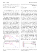
As Q1D is an initial value code, it needs a one- dimensional plasma equilibrium to begin. A plasma equilib- rium is generated using a TAE one-dimensional Grad Shafranov solver34 in conjunction with experimental param- eters. The equilibrium density and temperature profiles are shown in Fig. 5, where the blue lines represent the numerical density and electron temperature profiles and the red dots with error bars represent the experimentally measured values.
It is difficult to simulate increasing shine-through from
neutral beams that are injected away from the mid-plane as
well as higher scrape-off layer (SOL) magnetic field effects
self-consistently with a one-dimensional radial transport
code such as Q1D. These effects are modeled by artificially
enhancing the shine-through calculated in the MC code to
match with the experimentally observed shine-through.
Similarly, effects of enhanced parallel confinement are
mocked by directly reducing the parallel transport by a factor
of two. Finally, the axial contraction rate required for Q1D
to include axial compression effects is directly taken from an
experimental estimate of the axial length. With the given
equilibrium, the plasma transport coefficients are fixed at the
start of simulation and the transport equations are advanced
in time to match the experimental results. The transport coef-
ficients evolve as the FRC parameters change in time due to
the prescribed functional forms. With the local Bohm resis-
tivity and Bohm electron thermal conductivity model (i.e.,
fgB 1⁄4 fvB 1⁄4 1) and classical ion thermal conductivity, the e
simulated plasma decays too fast. The fast resistive decay
Phys. Plasmas 23, 052307 (2016) TABLE I. Transport coefficient used for simulating C-2 plasma.
cl
results in large Ohmic and compressional heating terms in
the electron energy equations, which further increase the
electron temperature and hence higher Bohm diffusion. Even
with fgB 1⁄4 0:1; 0:3 and fvB 1⁄4 1, plasma lasts less than 100 ls e
which is an order of magnitude smaller than the experimen- tally observed lifetime without neutral beams. With neutral beams, the plasma duration ranges from 3 to 5ms. This means that the resistive diffusion value required to simulate the experimental observations is much less than local Bohm’s diffusion. In these short time scales, neutral beams do not play any role in the evolution of the discharge. For the remainder of the paper, we will focus on the numerical results for the model of classical transport coefficients multi- plied by a fixed constant parameters as given in Table I. These coefficients have been chosen by minimizing the dif- ference in the numerical and experimental observables. Even though these multiplication factors may be regarded as phe- nomenological, they may be consistent with the underlying physics and experimental observations. Due to large ion orbits, the dimensionless ratio s 1⁄4 a=qi is close to unity for C-2, i.e., ion orbits span the whole plasma radius. Finite orbits have a stabilizing effects on ion turbulence35–37 and, hence, result in reduced transport. For electrons, Larmor radius is small and hence se 1⁄4 Ls =qe , where Ls, the turbulence shear scale length, is many times the electron Larmor radius. Thus, the multiplication factor is much greater than unity. These coefficients are consistent with the experimental observation of only low level electron scale turbulence in FRC core measured using multi-channel Doppler Backscattering.38
Comparison of simulated results to experimental meas-
urements for excluded flux radius measured using magnetic
probes at the wall, electron and ion temperature, and line-
integrated electron density are shown in Figs. 6–8. The
Multiple times classical f cl 1⁄4 5
Resistivity
Electronthermalconductivity fvecl1⁄420 Ion thermal conductivity fvi 1⁄4 1
g
excluded flux radius is calculated using the formula
pffiffiffiffiffiffiffiffiffiffiffiffiffiffiffiffiffiffiffiffi
FIG. 5. Profile of electron temperature (top) and density (bottom) that initi- alizes Q1D transport simulation (blue line: numerical; red dot with error bar: experimental).
rD/ 1⁄4 rw 1 B0=Bp, where B0 is the vacuum magnetic field, Bp 1⁄4 B0 þ dB is the total magnetic field measured at the wall in the presence of FRC, and rw is the wall radius. This
FIG. 6. Comparison of simulated excluded flux radius (RD/ in blue) with the measured one (in red). The separatrix radius (Rs where w 1⁄4 0 in green) is smaller than the excluded flux radius.