Page 2 - Diagnostic suite of the C-2U advanced beam-driven field-reversed configuration plasma experiment

11D815-2
Magee et al.
Rev. Sci. Instrum. 87, 11D815 (2016)
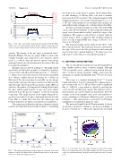
FIG. 1. Top: (left y-axis, black) neutral density measured with the FIGs; (right y-axis, red) neutral beam current. Bottom: signal on the neutron de- tector for a shot with gas (black solid) and a shot without gas (blue dashed).
current). The density of the gas target is measured with 3 Granville-Phillips 355 fast ion gauges (FIGs) located at the vacuum boundary and operated in a low emission current mode, Iem = 80 μA. Since the injected current, beam energy and target density are all well-measured, the neutron flux can be accurately calculated.
Example data are plotted in Figure 1. The high neutral gas density, plotted in the top panel, is obtained by opening a solenoid valve with 90 psi deuterium gas from t = 10 ms to t = 40 ms. A second set custom, fast solenoid valves are pu↵ed at t = 40 ms to further increase the density. At t = 50 ms, an NB is fired. Two shots are taken for each NB, one into the gas target and the other into the empty vacuum vessel. Because the shine through of the beam in the gas target is nearly 100%, in each case, the number of beam particles striking the far wall is the same, and the signal from the “no gas” shot can be simply subtracted from the gas shot signal to isolate the beam-gas component. (The slight increase in the signal during the no gas shot is presumed to be due to deuterium deposition by the beam. This is a small e↵ect and since the beam-in-gas and beam-in-wall shots are taken consecutively, it is neglected.)
The main practical di culty with this technique is that the neutrons are emitted from an extended volume, so calculating
the neutron rate at the detector requires 3D modeling. Here, we take advantage of a Monte Carlo code used to simulate fast ions in the C-2U geometry.11 By setting the magnetic field and plasma density to zero and the neutral density to n0 = 1.5 ⇥ 1014 cm 3 in the simulation, we can employ the existing code and synthetic neutron diagnostic to calculate the predicted flux.
In order to check the calculation, we fire each of the 6 NBs one at a time. Plotted in Figure 2 is the background subtracted signal versus beam number scaled to match the output of the simulation. The signal on each detector is largest when its nearest beam is fired, as expected. The resulting calibration factor (for the nominal PMT bias setting of detector 1) is 2.4 ± 1.4 ⇥ 107 n/s/V.
The main uncertainty in this method is the e↵ect of the NB on the gas density. The neutral gas density is measured at the edge of the vessel, and the gas density in the beam path may be lower due to neutral depletion.12 For this reason, it is important to verify with a second calibration method.
IV. NEUTRON SOURCE METHOD
The second calibration method uses an Americium Beryl- lium (AmBe) neutron source of known strength. Although 252Cf is typically used to calibrate fusion neutron detectors due to its narrow energy spectrum,5 AmBe sources have the advantage of a much longer half-life than 252Cf (433 yr versus 2.6 yr).
The source is a standard Amersham X.14,13,14 6 cm in length with radius 1.5 cm. It contains 10 Ci of alpha activity to give a neutron rate of 2.1 ⇥ 107 n/s. There is also a significant flux of ⇠100 keV -rays which we shield by enclosing the source in a 0.5 cm thick lead capsule. The shielded source is then mounted onto a probe which was inserted into the C-2U vacuum vessel from multiple entry ports and translated to create a distribution of 50 unique calibration points, as shown in Figure 3. (The interpolation is performed via Delaunay triangulation, for illustration purposes only.)
The measured signal from all 50 measurement locations are plotted as a function of distance to the detector in Figure 4. It can be seen that for r > 50 cm, the signal looks very much
FIG. 2. The background subtracted neutron signal as a function of the beam number is scaled to the Monte Carlo calculated neutron rate for both neutron detectors to obtain the calibration factors.
FIG. 3. A contour plot shows the signal strength as measured by neutron detector 1, located at the red star. The white triangles show the location of the source for each measurement, along the insertion path from each of 4 entry ports.