Page 3 - untitled

5582 Vol. 55, No. 21 / July 20 2016 / Applied Optics
Research Article
Initially, optimum coupling coefficient of ∼15% was expected [16], and 250 lines per inch (LPI) meshes were chosen for the output coupler to have minimum transmission below 10% to ensure the access of originally expected optimum coupling. In the lab test, it was found that the optimum coupling is ∼35% (discussed below). In order to reduce the tuning curve (blue) slope near optimum coupling, lower density 120 or 150 lines per inch meshes are used, which achieved much more stable laser performance than the original coupler when the spacing between the meshes drifts. Lower line density meshes cannot be used, as the mesh periodicity must be smaller than half- wavelength to avoid diffraction loss.
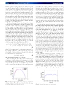
The other advantage of the new laser design is that the gain of the laser can be determined by varying the coupling coeffi- cient of the output coupler and, in the meantime, measuring the laser output power using an Ophir’s 3A-P-THz power me- ter. The aperture of the power sensor is 12 mm in diameter, which is smaller than the laser beam diameter. Therefore, a lens made of high-density polyethylene (HDPE) with a focal length of 150 mm is used to focus the laser beam onto the power sen- sor. Each time the output coupler coupling coefficient is changed by adjusting the parallel mesh spacing, the laser is optimized by tuning the cavity length before the output power is measured. The direct readings from the power meter are plotted as a function of coupling coefficient, as shown by the circles in Fig. 5. The solid curve in Fig. 5 is a best fit of the data using the modified Rigrod model [16]:
1∕4
P S·Is ·T 1−Li f2g0L ln 1−Li 1−T g ;
2 1 1−T 1∕2 1− 1−Li 1∕2 1−T 1∕2 (1)
where P is the output power, I is the saturation intensity, T is s
the coupling coefficient, Li is the total cavity loss, L 1.6 m is the length of the laser cavity, g0 is the gain of the laser, and S is the effective cross sectional area:
S 0.555·π·d2∕4; (2)
and the waveguide diameter is d 38 mm.
From curve fitting the data in Fig. 5, it is found that the gain
of the laser is 3 dB∕m, which is close to the gain of 3.15 dB∕m directly measured in the amplifier setup [17]. This gain is high compared with typical value of ∼1.1 dB∕m in reported laser works [16] and is near the high end of theoretical expectations
Fig. 5. Measured laser output power (circles) as a function of coupling coefficient. The solid curve is a best fit of the data using the modified Rigrod model described in [16].
[10]. When the coupling coefficient is tuned to near lasing threshold, the term inside the curl bracket in Eq. (1) is zero. For any fixed cavity loss, higher threshold coupling (closer to unity) means higher laser gain. The measured high threshold coupling coefficient of ∼90% in Fig. 5 is a direct indication that the laser has very high gain. In lower gain lasers, lasing action will cease at lower threshold coupling (∼35%) [16]. As shown in [17], the gain sensitively depends on pump level. This is confirmed in lab tests, as the high gain and high output power are measured after the CO2 pump is optimized by fine tuning the dichroic mirror and the pump laser beam incident angle. In fact, this is what motivated the new laser design described above.
Note that the laser powers shown in Fig. 5 are direct read- ings from the laser power meter, which are smaller than actual laser output powers due to two major factors. First, the 3A-P-THz power sensor absorbs 82.3% of the incident power at the laser frequency of ∼0.7 THz [18]. Second, the absorption and reflection loss of the HDPE lens need to be corrected. The absorption coefficient of the lens material HDPE is 0.235 cm−1 at 0.7 THz, while the refractive index is 1.538 [19]. The lens thickness is 1.7 cm at the center and 0.32 cm at the edge, with a radius of curvature of 7.85 cm. It is placed at where the Gaussian beam 1∕e intensity diameter is d 1∕e ∼ 2.14 cm. Calculations show that the lens power absorption coefficient is 28.5% and the reflection coef- ficient is 8.8%, which yield a lens transmission coefficient of 0.652. The above factors give a correction factor of 1.86 for the laser power. For the maximum power reading of 27.4 mW, the actual power is 51 mW. This is obtained with a CO2 pump laser power of 29 W at a wavelength of 9.27 μm. Therefore, the conversion efficiency is 16.4% of the Manley–Rowe limit [20], which says two pump photons are required to excite two lasing molecules to the upper energy level to obtain one laser photon output.
The optimum operation gas pressure is found to be ∼110 mTorr using a model 722B Baratron gauge (0–2 Torr range) from MKS Instruments. Other factors affecting laser power include ambient temperature and laser operation tem- perature, electric power stability, optical feedback to the laser cavity, etc. For all tests in the lab, the chiller (Model HRS024 from SMC) temperature is controlled at 15 0.1°C · 1.5% laser power stability is achieved over short time periods, as shown in Fig. 6. Over a longer timescale (∼10 min ), the CO2 laser cavity drift will cause small change in pump laser frequency, which will significantly change the pump efficiency
Fig. 6. Recorded laser power over 100 s period.