Page 7 - Inference of field reversed configuration topology and dynamics during Alfvenic transients

NATURE COMMUNICATIONS | DOI: 10.1038/s41467-018-03110-5
ARTICLE
0.4 0.3 0.2 0.1
0 0.4
0.3 0.2 0.1
0 0.4
0.3 0.2 0.1
0 0.4
0.3 0.2 0.1
0
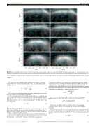
Fig. 6 FRC poloidal flux contours. Flux contours (cyan) superimposed with surfaces of equal emissivity from the 3d→3p oxygen 4+ transition (grey scale). Maximum emissivity is shown in white, while no emissivity is represented by black. The flux contour levels corresponding with 0 Wb (separatrix) and 0.01 Wb are labelled to show how flux expands in the open field region as the discharge evolves. The region of peak emissivity approximately tracks the flux expansion
If ψi;Biz are the flux and field profiles determined at positions zi along the internal wall of the vacuum vessel with radius r = Rw, the excluded flux radius profile is defined as
measurements in D. These are arranged into a probability distribution p(X|D) termed the posterior. A likelihood probability distribution p(D|X) measures the misfit between the model predictions H(X)and the measurements D. The probability of the spatial variable p(X) prior to taking any measurements is termed the prior probability distribution. According to Bayes theorem14, the posterior can be obtained from the likelihood distribution and the prior as
pðXjDÞ 1⁄4 pðDjXÞpðXÞ : ð15Þ pðDÞ
The term in the denominator p(D) is called the evidence (or marginal likelihood) and normalizes the volume of the posterior distribution to 1.
pðDÞ 1⁄4 R pðDjXÞpðXÞdX: ð16Þ
Given prior and likelihood, the most likely solution is the maximum
a posteriori (MAP) estimate, the solution in the posterior with the highest probability.
In the particular case where the forward model is linear, the spatial variable X(r) can always be discretized on a fine grid of dimension k, and a matrix K 2 Rn ´ k can be used to relate the discretized variable X 2 Rk with a set of n measurements in D2Rn
D 1⁄4 KX þ ε ð17Þ
sffiffiffiffiffiffiffiffiffiffiffiffiffiffiffiffiffiffiffiffiffi
i ψi
Rψ 1⁄4Rw 1 πR2Bi:
wz
ð13Þ
t=1.0 ms
t=2.0 ms
t=3.0 ms
t=1.5 ms
t=2.5 ms
t=3.5 ms
t=4.0 ms
–0.6 –0.4 –0.2 0 0.2 0.4 0.6 –0.6 –0.4 –0.2 0 0.2 0.4 0.6
t=4.5 ms Z (m) Z (m)
The position of the plasma mid-plane can then be estimated from the position where the excluded flux radius has its maximum.
A first-order approximation for the FRC separatrix radius is to consider it equal to the excluded flux radius at the mid-plane. A first-order approximation for the FRC x-point position is taken as the point along the axis Z2/3 where the excluded flux radius has fallen to 2/3 of its value at the mid-plane28. The FRC length is then approximated by
L 1⁄4 2Z2=3: ð14Þ
Bayesian inference of GPs. Bayesian inference is used in this paper to calculate the posterior distribution of currents given the magnetic measurements. The method, however, is generic enough to be used in a variety of related tomographic problems, which can be stated as follows.
Given a forward model D = H(X) relating a continuous variable X(r) function of location r = (r1,r2,r3) with some discrete set of measurements in the data vector D, the objective is to obtain all the solutions for X(r) that can explain the
NATURE COMMUNICATIONS | (2018)9:691 | DOI: 10.1038/s41467-018-03110-5 | www.nature.com/naturecommunications 7
0.01
0.01
0.01
0.01
0.01
0.01
0.01
0.01
R (m) R (m) R (m) R (m)
0
0
0
0
0
0
0
0