Page 8 - Inference of field reversed configuration topology and dynamics during Alfvenic transients

ARTICLE
NATURE COMMUNICATIONS | DOI: 10.1038/s41467-018-03110-5
0.35 0.3 0.25 0.2 0.15 0.1 0.05
a 4.5 4 3.5 3 2.5 2 1.5 1 0.5
b 50 c 45
40 35 30 25 20 15 10
0.3
2.5
2
1.5
1
0.5
300
60
5 000
Assuming additive Gaussian measurement noise ε = N(0,ΣD) independent of X, the likelihood function can be modelled by an n-dimensional Gaussian distribution
ð18Þ
where ΣD 2 Rn ´ n is the data covariance matrix.
The prior distribution can also be approximated by a multivariate probability
As the dimension k of the multivariate normal distribution is made increasingly large, the multivariate normal distribution approaches a continuous distribution, and at this limit a GP is obtained15. In our case, the vector X becomes a continuous function X(r) of the spatial location. All possible solutions for X(r) can then be thought of as being generated by a stochastic process, described by the corresponding GP.
For a large number of situations in plasma physics, transport processes will work in the direction to reduce the spatial gradients of X(r). In other words, our prior belief about X(r) is that it must be a smooth function of r. The prior covariance kernel required for the inference can then be parameterized using the Squared exponential (SE) function, which is one of many options available15 to model the spatial correlations between the values of a smooth profile variable at two points r and r':
1 1 pðDjXÞ 1⁄4 exp ðD KXÞTΣ 1ðD KXÞ
def
250
150
100
50
50 200 40
0
12345 12345 12345
00
t (ms) t (ms) t (ms)
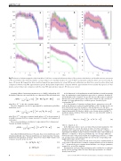
Fig. 7 Inference of plasma magnetic related variables. Solid lines correspond with mean values of the posterior distribution, and shaded areas are a measure of the uncertainty of the inferred variables corresponding to one standard deviation for shot # 48269. a Separatrix radius Rs (blue) and o-point radius R0
pffiffiffi
times 2 (green). b Trapped flux (blue) and the trapped flux approximation for a long FRC (green). c Machine axis Bz at the o-point z position (blue) and
comparison with the long FRC approximation (green). d Separatrix length (blue) compared with the approximation from excluded flux (green). e Total plasma current (blue) and comparison with the long FRC approximation (green). f Total vessel current
30 20 10
ð2πÞn=2 jΣD j1=2 2 D
distribution over X
pðXÞ1⁄4 1 exp 1ðX μ ÞTΣ 1ðX μ Þ
where ΣX 2 Rk ´ k is the prior covariance kernel and μX 2 Rk is the prior mean. It is usually convenient (but by no means necessary) to consider a zero mean μX = 0 on the prior.
The posterior distribution can likewise be approximated by a k-dimensional Gaussian probability distribution.

ð2πÞk=2jΣXj1=2 2 X X X
ð19Þ
ΣXðr; r′Þ 1⁄4 σ2exp 2 2 2

1 ðr r′ÞTΛ 1ðr r′Þ ð23Þ 2
1 1 pðXjDÞ1⁄4 k=2 1=2 exp 2ðX μÞTΣ 1ðX μÞ :
ð2πÞ jΣj
ð20Þ
with Λ 1⁄4 diag λ1;λ2;λ3 .
In the Bayesian context, σ and λi are termed the prior hyper-parameters. The
Since all probability distributions are Gaussian, the posterior distribution can be obtained analytically, since Gaussian distributions are transformed into Gaussian distributions through linear operations. The posterior mean (MAP estimate) and covariance are given in this case by11:
standard deviation σ controls the spread of values of X. The scale length λi determines how quickly the plasma variable can change with the coordinate ri. A large length scale will give a large covariance between the values of the variable X at different ri coordinates, so the prior probability (Eq. (19)) for large differences between the values of the plasma variable X at neighbouring positions ri ; r′i will be low. In other words, if the plasma profiles are smooth, the corresponding scale lengths will be large, and vice versa.
The SE kernel is by no means the only choice for a prior covariance kernel. A good review of GPs and the most common covariance kernels used can be found in ref. 15. In general, the prior covariance kernel will have a set of hyper-parameters, arranged in a vector θ for simplicity.
Determination of the prior hyper-parameters can be considered as a continuous model selection problem, where the more likely hyper-parameters are obtained directly from the data31.
8
NATURE COMMUNICATIONS | (2018)9:691
| DOI: 10.1038/s41467-018-03110-5 | www.nature.com/naturecommunications
T 1 1 1 Σ1⁄4KΣDKþΣX ;
μ 1⁄4 ΣKT Σ 1 D: D
ð21Þ ð22Þ
L (m)
R (m)
Ip (kA)
0(mWb)
I (kA) v
Baxis(mT) min