Page 5 - Demo

022503-5 Steinhauer, Berk, and TAE Team
Phys. Plasmas 25, 022503 (2018)
source rate is ignored so that sinv 1⁄4 sN. becomes
1d vdn! n rn 1⁄4k2
Then, Eq. (6)
(7)
r dr vn;s dr ‘2i
k2 􏰆 ‘2i 􏰈ZM1􏰃1􏰉; r􏰅Rs;
vn;s Zs sjj sN
where vn,s denotes the separatrix value. Once the “eigenvalue” k is found, the end-loss time follows by solving Eq. (7b) for sjj. Equation (7) is, in fact, an eigenvalue prob- lem because the second-order equation (7a) has three bound- ary conditions: at r 1⁄4 Rs, n 1⁄4 ns, and (dn/dr)s 1⁄4 ns/Ln,s, while at the radial wall boundary, vndn/dr ! 0 (no flux through the wall).
1. Solutions
Equation (7) has an analytical solution in the reduced case of flat particle transport rate vn 1⁄4 vn,s 1⁄4 const and the slab approximation (drop the 1/r and r factors in the deriva- tive term). Then, the density profile is exponential, n1⁄4nsexp[–(r–Rs)/Ln,s], and the eigenvalue is k1⁄4‘i/Ln,s. However, the numerical integration of the more general sys- tem is straightforward if the particle transport rate is express- ible as a function of the density. More realistically, the transport rate varies with parameters. For example, if the particle transport rate has a power-law dependence, vn 1⁄4vn,s(n/ns)a. This too has an analytical solution, and the eigenvalue is k 1⁄4 (1þa/2)1/2‘i/Ln,s. The Appendix considers relevant values of a, yielding numerical results close to the analytical result. For classical particle transport, k 􏰂 1.17‘i/ Ln,s, and for Bohm transport, the factor is slightly lower (1.12). Since in fact vn 􏰁 na/B2, a more realistic solution accounts for the effect of finite-b in the SOL. This requires a modest numerical computation and yields a higher value
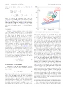
FIG. 4. Interpreted end-loss time referenced to free-streaming time.
C-2U point, which has an interpreted end-loss time sjj 1⁄4 2.4 ms; this notably exceeds the ion-ion scattering time of sii1⁄40.73ms. For mirror-confinement (empty loss cone), smir 􏰂 siilnRM, where RM is the mirror ratio. If RM 1⁄4 15, then smir1⁄42.0ms, which is comparable to the inferred 2.4ms value. The C-2U experiments employed a “plug” mirror with RM in this range.5 Thus, the interpreted end-loss time is com- parable to the mirror prediction. In view of the long mean-free path, the empty loss cone prediction is more realistic than the collisional “full loss-cone” expression smir 􏰁 sfsRM 􏰁0.22 ms.
Historically, nearly all FRX experiments have employed little or no magnetic mirrors at the ends of the main confine- ment coil system. Weak mirror ratios, 􏰁1.1 or less, were applied mainly to the center of the FRC at the mid-plane of the coil system. The lone exception before the construction of C-2 and C-2 U was in the FIX facility24 which had a mir- ror ratio of 􏰁2–3. Using the “two-point-equilibrium” inter- preter,21 the end confinement ratio for the FIX example is sjj/ sfs 􏰁 1.5. This is slightly above the blue band in Fig. 4 and about even with the lowest C-2 values (labeled with red “􏰄” symbols). The C-2 and C-2U facilities have a mirror ratio of about three at the end of the main confinement vessel (Fig. 1). In early C-2 experiments, sjj/sfs was similar to FIX. The large increase in end confinement during the subsequent evolution of C-2 and C-2U clearly arose from techniques added over a period of time: neutral beam injection, divertor biasing, increased field in the formation sections during the confinement phase, and plasma hygiene measures. The phys- ical reasons for increased sjj/sfs are the subject of specula- tion, the most likely candidates being the improved stability of the main (FRC) plasma and the extended SOL regions improving the effectiveness of the plug mirror (not shown in (Fig. 1) and reduced neutrals.
IV. COUPLED PARTICLE TRANSPORT EXPRESSIONS
Once a fix is gained on the companion transport rates, vn,s and 1/sjj, one can proceed to an equation that combines
k 1⁄4 1.53‘i/Ln,s. Once k has been determined, time follows from solving Eq. (7) for s
the
end-loss
jj s1⁄4ZM=Zs: (8)
jj k2vn;s=‘2i þ1=sN C. Interpretation of FRC database
Apply Eq. (8) to the FRC data compendium.21 It is use- ful to compare sjj with the nominal inertial (free-streaming) time of a fluid
sfs 1⁄4 ZMðmi=kTtÞ1=2: (9)
Figure 4 portrays the ratio sjj/sfs vs maximum total tempera- ture Tt. The blue band reflects the range of interpreted values for traditional FRCs, in which sjj lies in the range of (0.6–2.5)sfs. The C-2 and C-2U results, however, depart rather abruptly from the inertial trend. The black dashed line in the figure is the ion scattering time sii (referenced to sfs). Accounting for pressure balance, its scaling is sii/sfs 􏰁 Tt.3 The symbols approach this line. Notice especially the lone