Page 15 - Positional stability of field-reversed-configurations in the presence of resistive walls

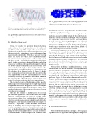
FIG. 22. Comparison of linear and non-linear closed loop simula- tions near the predicted maximum latency of 13 cycles (130 μs).
not plotted, the agreement for latencies of 8 and 9 cycles is equally good).
FIG. 23. A more realistic model of the conductiving wall surround- ing an FRC. Compared to an axisymmetric wall, the 3-D structure changes the instability growth time from 405 μs to 75 μs
linear model, but need to be taken into account when at- tempting to extrapolate results.
For example, it is not clear if the correct rigid volume for modeling an axial instability will also be the right choice for modeling a radial instability. If the rigid volume has phys- ical significance, this would be the case. But if it is merely a proxy for some other energy dissipation (or collection) mechanism, a different scaling may be neccesary for dis- placement in a different direction. Testing this hypothesis would require simulations using a non-linear, hybrid 3-D code that at this point in time does not exist.
Nevertheless, the absence of such a code also makes the linear model the currently best available option to reason about radial instabilities. Therefore, it is reassuring that even though there is no direct evidence from simulations that the linear model will make correct predictions for radial instabilities, all the testable assumptions of the underlying theory have been validated, and there is no evidence that the remaining assumptions would prove incorrect for radial displacements.
When used for modeling of axial displacements, the lin- ear model has the obvious advantage of being significantly faster to calculate. In addition to that, however, it also al- lows to incorporate the effects of a three dimensional wall – something that is not possible when using an axisymmetric, non-linear code. The effects of a more realistic wall can be profound. Figure 23 shows a three dimensional model of a realistic FRC vacuum chamber with diagnostic ports as well as neutral beam cutouts. Otherwise the geometry, resistivity and thickness is similar to the axisymmetric wall shown in figure 4. The two walls also have similar characteristic L/R times: the slowest eigenmode decays with a time constant of 1.6 ms (3-D model) and 1.2 ms (axisymmetric model). However, the growth rate of the axial stability changes from 405 μs (axisymmetric wall) to 75 μs. This is because the 3- D model has large cutouts in the central area, where move- ment of the plasma would otherwise excite the largest eddy currents. This difference is not visible in the L/R time of the wall, because the eigenmodes simply shift to a different lo- cation.
D.
Suitability of linear model
Overall, we consider the agreement between the linear and non-linear closed loop simulations to be sufficiently good for control algorithm design. The linear model re- produces the global behavior of the controlled system (am- plitudes, periods, return times) over a wide range of pa- rameters and scale lengths. While there are some discrep- ancies for longer cycle times, these can be fixed by us- ing a more accurate representation of the control coils in the linear model. Generally, the predictions of the linear model tend to overestimate the instability drive, which in- creases the confidence that algorithms designed for the lin- ear model will also stabilize the non-linear system. How- ever, we also found a single, so-far unexplained failure of the linear model for a specific, insulated set of parameters (gain 25, cycle time 10 μs, latency 6 cycles, cf. figure 21). In this case the linear model underestimates the saturated oscilla- tion amplitude by about 50%. This emphasizes the need to eventually test every algorithm in a non-linear simulaton, but appears to be sufficiently rare to justify doing the ma- jority of the design work using the linear approximation.
The good performance of the linear model also provides further support for the assumption of a rigid displacement. If significant amounts of energy were stored or freed by de- formations, the linear (rigid) model would be unlikely to re- produce the behavior of the system over the range of param- eters that we investigated.
That said, the evidence of rigid behavior does not im- ply a physical significance of the rigid volume (the free pa- rameter). Mathematically, the choice of the rigid volume amounts to a scaling of the instability drive by defining an effective toroidal plasma current (which linearly affects the driving force, and quadratically affects the restoring force). Therefore, it is possible to derive the same mathematical model by assuming a very different rigid volume, and in- stead postulating the existence of an additional energy sink (e.g. by the displacement causing additional heating) that brings the effective instability drive to the same level. These considerations do not affect the practical usefulness of the
E.
Experimental Implications
While we deliberate made no attempt at developing an optimized control algorithm, or using physical diagnostics
15