Page 13 - Positional stability of field-reversed-configurations in the presence of resistive walls

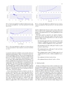
FIG. 14. Period and amplitude for different feedback gains in lin- ear, closed-loop simulations. Cycle time and latency were held fixed at 10 μs.
FIG. 15. Period and amplitude for different cycle times in linear, closed-loop simulations. Gain was fixed at 25, latency was held at one cycle.
is reached at which the feedback system switches between minimum and maximum voltage on every cycle. Slower cy- cle times and higher latencies increase both amplitude and period of the stabilized position. All offsets (not plotted) are between -1 cm and +1 cm with no clear dependency on gain or cycle time, and an approximately linear dependence on latency. Settling times (not plotted) are between 2.4 ms and 4.4 ms and show no clear dependence on any parameter (in- cluding gain). This may at first appear surprising, but with the above definition of settling time and amplitude, a sys- tem with higher gain will have smaller amplitudes and thus take longer until the position has returned to the amplitude window - countering the effect of an overall faster return ve- locity (due to the increased gain).
A more interesting observation is that for very fast cy- cle times and low latencies, the control algorithm starts to perform worse. This is because in this regime the coil cur- rents are shielded out by the resistive wall - the algorithm switches very quickly between positive and negative volt- ages, but the plasma feels almost no change in the mag- netic field. An obvious improvement to the control algo- rithm is to apply a filter to the coil currents before calculat-
FIG. 16. Period and amplitude for different latencies in linear, closed-loop simulations. Gain was fixed at 25, cycle time was fixed at 10 μs.
ing the weighted sum. However, in the context of this work we’re not interested in optimizing the algorithm but in the quality of the plant model so no such optimizations were attempted.
The linear model is expected to be valid for displace- ments up to 20 cm. From the results of the scan, we can therefore make the following predictions for the non-linear behavior of the system:
13
C.
• The minimum gain (with 10 μs cycle time and 1 cycle latency) to stabilize the system is about 7 (lower gains result in oscillation amplitudes of more than 20 cm).
• The maximum cycle time (with gain 25 and one cycle latency) is about 60 μs.
• The maximum latency (with gain 25 and cycle time 10 μs) is 13 cycles, i.e. 130 μs.
• The optimum gain is about 30 (higher gains do not significantly decrease the oscillation amplitude or pe- riod).
• The optimum cycle time is about 30 μs.
• The optimum latency is about 6 cycles, or 60 μs.
Non-linear results
Ideally, it would have been possible to include the results from non-linear simulatons as a second series of datapoints in figures 14, 15 and 16. Unfortunately this was not feasible because the limited simulation time available for non-linear simulations did not allow the derivation of unique values for most of the plotted quantities. This can be readily seen from e.g. figure 13: had the simulation been terminated at 6 ms (instead of extending until 30 ms), we would have ob- tained a quite different (and incorrect) value for the offset (and thus also a much larger amplitude). In principle, we could have continued the non-linear simulation until after 6 ms, but in this case the (slow but steady) changes in the