Page 14 - Positional stability of field-reversed-configurations in the presence of resistive walls

14
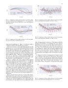
FIG. 17. Comparison of linear and non-linear closed loop simu- lations near the predicted minimal gain of 7. (The near-perfect agreement with gain 10 is most likely due to chance and disappears again at gain 20.)
FIG. 18. Comparison of linear and non-linear closed loop simula- tions near the predicted optimum gain of 30.
unperturbed equilibrium (cf. figure 1) would have made a comparison with the linear predictions pointless.
Instead, we therefore look at individual simulations with parameters close to the thresholds predicted by the linear model. When looking at these plots, it is important to keep in mind that each simulation runs independently in its own closed loop with a non-linear feedback algorithm, so mi- nuscule changes in plasma state can cause huge differences in the applied voltage. Therefore, corresponding simula- tions are not expected to result in matching graphs, but should rather have similar global characteristics (like oscil- lation periods, saturated amplitudes, or return time).
Figure 17 compares the results of linear and non-linear simulations near the lower gain threshold of 7. Oscillation period and amplitude agree. However, there is insufficient data to determine if the non-linear simulations will go un- stable, or settle into a stable, large-amplitude oscillation.
If we look at the results near the predicted optimum gain of 30 (figure 18), we find a similar situation. The initial evo- lution is predicted reasonably well, and arguably a gain of 40 does not improve upon a gain of 30, but the low number of (global) oscillations in the simulated time range makes it difficult to make statements about saturated amplitudes or frequencies.
Figures 19 and 20 show results close to the predicted max- imum stable cycle time of 60 μs, and optimum cycle time of 30 μs. Here we find that the linear model significantly over- estimates the saturated amplitudes and oscillation periods for cycle times of 35 μs and above. For cycle times below this
FIG. 19. Comparison of linear and non-linear closed loop simula- tions near the predicted maximum cycle time of 60 μs.
FIG. 20. Comparison of linear and non-linear closed loop simula- tions near the predicted optimum cycle time of 30 μs.
value, the agreement is satisfactory. This indicates that the predictions from figure 15 are qualitatively correct, but the dependency is not as strong as the linear model indicates. The most likely explanation for this is the representation of the control coils: in the linear model, they are represented as thin filaments, while in the non-linear simulation they have finite extent and volume currents. This leads to a dif- ference in the self inductance, and thus a difference in the currents that becomes bigger as the cycle time becomes big- ger.
Looking at the effects of varying latencies (figures 22 and 21), we find good agreement for all latencies other than a value of 6 cycles. For this specific number, the linear pre- diction of the saturated amplitude is much smaller than the non-linear value. The reason for this discrepancy is not clear, and it seems to be specific to this specific value (while
FIG. 21. Comparison of linear and non-linear closed loop simula- tions near the predicted optimum latency of 6 cycles (60 μs).