Page 6 - Positional stability of field-reversed-configurations in the presence of resistive walls

ρf is the fast ion charge density, P is the plasma pressure, ν is the viscosity, and f2 is a source term due to collisions, charge exchange, and fast ions becoming part of the fluid. The equation for the neutral fluid has the same form, but without the B⃗ and E⃗ terms.
The electric field E⃗ is given by Ohm’s law,
E⃗ = −⃗u × B⃗ + η⃗jp + f3 (35)
where η is the plasma resistivity and f3 due to collisions be- tween fast ions and (fluid) electrons.
The plasma pressure P is determined via the total energy w by
P n∥⃗u∥2
w=γ−1+ 2 (36)
B.
Initial Conditions and Unperturbed Evolution
γ P n ∥ ⃗u ∥ 2 ⊥ ∥
Both linear and non-linear simulations have been started from the same initial conditions. These conditions were ob- tained by starting with an arbitrary MHD equilibrium and letting the (non-linear) simulation run until a steady-state was achieved. The equilibrium magnetic field was in the or- der of 600 G with a mirror ratio of 3.3.
Simulations have been run with a mesh resolution in the order of 1 cm2, a viscosity ν = 200 kg/sm to ensure numerical stability (fluid time steps are in the order of 10−7 seconds) and three times Spitzer resistivity. The anomalous resistiv- ity is a substitute for the absence of multiple ion species and necessary for a non-zero Okawa current drive. The value has been chosen to match experimental results in the C-2U device. Thermal conductivities are classical but calculated with a density floor of 1 · 1018 m−3 to avoid unrealistic con- ductivities in the low-density regions.
Current drive and heating are provided by 6 neutral beams injecting 7 MW of 15 keV particles. The point of clos- est approach to the machine axis is at z = ±30 cm with im- pact parameter (i.e., radius) 19 cm. At this point, the parti- cle trajectory is angled 15 degrees off the toroidal direction (i.e., the particle source is displaced axially from the point of closed approach).
In experiments, long-lived FRCs are re-fueled by cryo-
genic pellet or compact toroid injection. Q2D does not
yet have full support for these methods, so fueling was
instead Either of those causes transient, large perturbations XXXXXXXXXXXXXXXXXXXXXXXXXXXXXXXXXXXXXXXXXX
∂ w
∂t =−∇· γ−1+ 2 ⃗u+⃗u·(⃗jp×B⃗)
6
+kB∇· κi ∇⊥+κi∇∥ Ti (37) +k ∇· κ⊥∇ +κ∥∇ T
Be⊥e∥e + η ∥ ⃗j p ∥ 2 + f 4
Here γ is 2/3, kB is the Boltmann constant, κ is the thermal conductivity (with subscripts for parallel/perpendicular and electrons/ions), T is the temperature (for elec- trons/ions), and f4 is a source term from collisions, charge exchange, and particles falling under the energy threshold. The electron temperature is determined by
(38)
of the plasma equilibrium. In order to be able to separate
n 1∂+⃗ue+∇·⃗uT= eee
XXXXXXXXXXXXXXXXXXXXXXXXXXXXXXXXXXXXXXXXXXXXXXXXX

evolution of the instability from perturbations due to
⃗2
+η∥jp∥ +νei(Ti −Te)+ f5
was provided by a hypothetical particle source inside XXXX
the separatrix that provided a flux continious stream of XXXXXXXXXXXXXXXXX
1019 neutrals per millisecond at a temperature of 800 eV.
In order to prevent the plasma from becoming axially un- stable, all unperturbed simulations were run with super-
conducting walls.
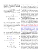
Figure 4 shows the flux contours and plasma current den-
sity after 1 ms when the simulation has reached an approx- imate steady state. Figures 1 and 2 show the evolution of separatrix radius and length and average separatrix den- sity and temperature over time. Figure 3 shows the evolu- tion of FRC “ellipticity”. This quantity gives a measure of how the separatrix trace (on a plane with fixed toroidal an- gle) compares to an ellipse with the same semi-minor axis and elongation. It is defined as the symmetric difference between the separatrix area and the ellipse’s area, normal- ized to the area of the separatrix, with the sign indicating the bigger of the two areas (a positive sign indicates that the separatrix area is larger than the area of the ellipse). The take-away from these figures is that global plasma parame- ters are relatively constant throughout the simulation. Fig- ure 5 shows the evolution of the axial stability parameter (Fzc in equation (10)). For this computation, fields from wall currents were considered part of the vacuum field, B⃗v (the reason for this will become clear in section IV C). Since
where f5 is a source term due to collisions with fast ions, ne=n+nfand⃗ue=n/ne⃗u−⃗jp/(ene).Theiontemperature Ti is calculated as the difference between the total temper- ature (obtained from pressure) and electron temperature:
P nf
T = k n −n Te (39)
bii XXXXX
P nf
T i = T − T e = k n − n ( +X 1 − T e ) (40)
bii XXXXXXXXX
XXXXXXXXXXXXXXXXXXXXXXXXXXXXXXXXXXXXXXXXXXXXXXXXX
γ−1∂t γ−1
− ∇ · κ ⊥e ∇ ⊥ + κ ∥e ∇ ∥ T e
fuelling, neither cryogenic pellets nor compact toroids

where used in simulations for this work. Instead, fueling
XXXXXXXXXXXXXXXXXXXXXXXXXXXXXXXXXXXXXXXXXXXXXXXXX
XXXXXXXXXXXXXXXXXXXXXXXXXXXXXXXXXXXXXXXXXXXXXXXXX
The neutral pressure Pn is given by Pn n∥⃗u∥2
wn = γ−1 + 2 (41) Pn
∂ w n
Tn = k n (42) bn
γ P n n ∥ ⃗u ∥ 2
∂ t = − ∇ · γ − 1 + 2 ⃗u (43)
+ kBnνn(T − Tn) + ∇ · (κn∇Tn) (with ⃗u and n referring to the neutral fluid).