Page 7 - Positional stability of field-reversed-configurations in the presence of resistive walls

7
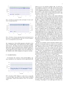
2.0 1.6 1.2 0.8 0.4 0.0
45 36 27 18 9 0
Length Radius
123456 Time [ms]
FIG. 1. Evolution of separatrix radius and length over time in ab- sence of any perturbations.
ulation at one, two and three milliseconds. In each case, any (midplane symmetric) wall eddy currents that existed at that time were “frozen in”, i.e. they were considered part of the equilibrium field and not subject to resistive decay. The resistivity of the wall was then changed from supercon- ducting to a realistic value, resulting in characteristic eddy current decay times in the order of 1.2 ms.
This procedure (initial evolution with superconducting walls followed by freezing of wall currents instead of using resistive walls from the beginning) was devised in order to be able to compare perturbed with unpertubed evolution. Had we skipped the settling period with superconducting walls, we still would have seen instability growth, but we would be unable to determine a corresponding axisymmet- ric equilibrium for linearization. Moreover, we would be un- able to distinguish if an incorrect linear prediction was due to non-linear behavior of the plasma (e.g. non-rigid move- ment), or simply because the axisymmetric equilibrium it- self was still evolving (so that the linearization around the initial equilibrium was no longer valid even before the in- stability had started to grow significantly). The use of super- conductivity during the settling phase was purely for com- putational convenience (and would thus not be required for e.g. experimental verification). An alternative, equivalent procedure would have been to use resistive walls from the beginning and instead implement an additional numerical “cleaning” scheme to eliminate any perturbations from ax- isymmetry.
Ideally, we would have ran the simulation until the insta- bility arose from numerical noise. However, we wanted to compare the evolution of the instability starting from mul- tiple, different points in time to rule out the existence of any internal plasma states that significantly affect plasma stability but whose evolution is not captured in figures 1 to 4. Therefore, the initial plasma state was explicitly per- turbed. The perturbation was a 1 cm axial displacement combined with the wall current excitation predicted by the linear model (using various choices of rigid volume).
Figure 6 shows an example time history of the axial sepa- ratrix location together with the least-squares fit to an ex- ponential function with unknown time constant. In this example, the initial perturbation was calculated using a spheroidal rigid volume with radii 46 cm/92 cm. The fitting results for a variety of initial conditions are plotted in fig- ure 7. This figure can be used to estimate the uncertainty in the time constants stemming from the choice of initial per- turbation and fitting window. Traces in the same color rep- resent different initial conditions - the initial perturbation has been calculated with three different choices for the rigid volume: a 46 cm/92 cm ellipsoid, a 50 cm/100 cm ellipsoid, and a 40 cm/80 cm ellipsoid. As one can see from figure 10, these correspond to linear predictions of the time constant from 50 μs to 500 μs. However, in the non-linear simulations the difference between least-square fitted time constants is only about ±5%, indicating that the effects of the initial per- turbation rapidly become irrelevant as the instability grows. A second source of uncertainty is the choice of time window for fitting. From figure 8, we would expect the time con-
300 240 180 120
60 0
4.0 3.2 2.4 1.6 0.8 0.0
T
n
123456 Time [ms]
FIG. 2. Evolution of mean separatrix density and temperature in the absence of any perturbations. The ratio of electron tempera- ture to ion temperature is about 60:200.
the computation of the stability parameter depends on the choice of rigid volume, it was repeated for a variety of plau- sible choices. The figure shows the minimum and maxi- mum value that was obtained when varying the rigid vol- ume from a spheroid that barely enclosed the separatrix to a large spheroid of minor radius 70 cm (10 cm distance to the chamber wall), while keeping the elongation constant.
C.
Perturbed Evolution
To determine the evolution of the axial instability, sep- arate simulations were branched off the unpertubed sim-
0.02 0.00 0.02 0.04 0.06
123456 Time [ms]
FIG. 3. Evolution of FRC “ellipticity”. A value of zero corresponds to a perfectly elliptic separatrix (when looking at a plane with fixed toroidal angle). Negative values indicate a more “race-track like” shape.
Ellipticity Temperature [eV] Length [m]
Density [1019m-3]
Radius [cm]