Page 8 - Demo

042504-8 Rath et al.
Phys. Plasmas 24, 042504 (2017)
The drawback of this approach is that the feedback con- troller can (by chance) suppress exactly those dynamics in which the models differ. To account for this, we ran simula- tions with a large number of different feedback controllers. We expect that the likelihood that each of those controllers hides exactly the same dynamics (and that those dynamics also happen to be exactly those where the linear and non- linear models differ) is negligible.
Furthermore, for our purposes, the comparison does not need to demonstrate a complete equivalence of linear and non-linear models. Rather, it is sufficient if the linear model correctly predicts the system stability and control power for the majority of cases. In this case, it can be used to efficiently derive and test the feedback controllers, whose ultimate per- formance can then be validated with just a few non-linear simulations.
In all closed-loop simulations, the perturbation was applied at 1 ms, and the control system was activated when the displacement reached 5.2 cm.
A. Control algorithm
The feedback control was simulated using 8 magnetic coils as actuators. The coils were located outside of the resis- tive wall at r 1⁄4 1:032cm and z 1⁄4 62:2m;61:7m;61:2m; 60:4 m (cf. Figure 1). Each coil had 20 turns and could be driven with a voltage of up to 61:6kV in steps of 400V (these choices correspond to the capabilities that were even- tually mandated for the control hardware of the C-2W device). As diagnostic, we used an artificial direct measure- ment of the separatrix centroid. In experiments, the plasma position will be inferred by an “observer” algorithm from the radiation center (as determined by axial bolometers) and the excluded flux radius centroid (as determined by magnetic measurements and flux loops). However, for the purposes of validating, the linear model including the observer algorithm in the simulation is not desirable because it would make it difficult to distinguish between the model validity limits and limitations of the chosen observer.
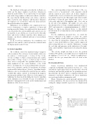
The control algorithm is depicted in Figure 6. The con- troller receives a “measurement” of the separatrix centroid and the current in each control coil. It then computes a weighted sum of each coil current, the axial separatrix loca- tion, and the axial velocity. This single scalar value is multi- plied with a coil-specific gain, which in this case is þ1 for coils on the right side of the midplane and 1 for coils on the left side of the midplane. The number for each coil is then interpreted as a voltage command, quantized to steps of 400 V, and saturated to a maximum/minimum of 61600 V. Finally, we impose an artificial latency (so that updated measurements do not immediately result in updated actuator commands).
For the simulations presented here, we varied the latency (expressed as the number of cycles), the control cycle time, and the overall (scalar) gain. As discussed before, we expect that by varying these parameters, we reduce the chance to miss model differences that could be suppressed when testing with just one controller. Furthermore, varying the cycle time and gain gives us the indications of the mini- mum control hardware requirements for keeping the plasma stable.
The velocity weight was kept at zero, the position weight at 500, and the coil weights chosen as (starting from the midplane) (7, 8, 6, 3) 10 2 A 1 (which is roughly propor- tional to the force per current that each coil exerts on the plasma).
B. Linear predictions
Linear, closed-loop simulations were implemented completely in Simulink. Linearization was done at t 1⁄4 1 ms and with the rigid volume that best reproduced the observed non-linear, uncontrolled growth rates for perturbations start- ing at this time. In order to allow a comparison with the (axi- symmetric) non-linear simulations, the linear simulations were performed with an axisymmetric wall.
Figure 7 illustrates the control input and output in a typi- cal linear simulation. The linear system was initialized by scaling the (unique) unstable eigenvector to a displacement
FIG. 6. Simulink model of the control algorithm used in closed-loop simula- tions. The green ports on the left are sources of synthetic measurements, and the cyan ports are a sink of actua- tor commands.