Page 5 - Rotational stability a long field-reversed configuration

032507-5
Rahman et al.
Phys. Plasmas 21, 032507 (2014)
FIG. 6. Radial profiles for the azimuthal-ion velocity, vih vs. r at six different times, at the mid-plane, z 1⁄4 0.
t 1⁄4 25 150 ls, during formation, equilibrium, and decay. As shown, the ions accelerate reaching a maximum velocity at t 1⁄4 75 ls, near the outer radius of the FRC. In agreement with Figure 6, the velocity profile establishes a sharp gradi- ent and reverses sign near the separatrix. The velocity profile after 50 ls is characteristic of a rigid rotor (RR), and remains RR-like as it decays from 2 107 cm/s to 5 106 cm/s.
In the FC-FRC experiments, the ion temperature and azimuthal-flow velocity are measured by Doppler spectros- copy of high-Z impurities added to facilitate measurement. The large gyro-radius for these impurities makes them more likely to exist in the outer region of the plasma. The simu- lated velocity magnitudes are of the same order as those measured by Harris et al.8
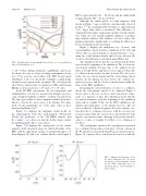
Figure 7(a) displays the mid-plane radial profile for the axial-magnetic field. The axial-magnetic field profile follows the prediction of the 1-D RRM, namely, that Bz / tanhðn n0Þ. Also note that the field is larger outside the null than inside, due to ion rotation.
Figure 7(b) displays the axial-profile for the radial- magnetic field, measured along the null-field radius of the FRC, with the appropriate change of polarity through z 1⁄4 0. From Figures 7(b) and 3, we estimate that the axial length of
FRC is approximately DL 80–90 cm, and the radial width is approximately DR 30 cm, at 100 ls.
Although the radial profile for axial magnetic field shown in Figure 7 agrees with the experimentally observed profiles,8,10 the maximum-field intensity is approximately 3–4 larger than what is measured. This difference is explained by the higher temperatures produced in the simula- tion, which does not include impurity radiation. A prelimi- nary analysis indicates that radiative loss does reduce the plasma temperature significantly, reconciling the differences between simulation and experiment.
Figure 8 displays the mid-plane ion-, electron-, and total-azimuthal current densities, simulated at 50, 100, and 150 ls. The ion current density is calculated from Ji 1⁄4 envih, using the actual plasma density and velocity, whereas the electron current density is calculated using Ohm’s law.
The simulation shows that the ion current density domi- nates from the beginning of the simulation. The electron cur- rent density initially develops due to the applied electric field, at 50 and 100 ls, and then reverses sign at 150 ls due to collisions between the ions and electrons. The effect is to reduce the ion current density and the total plasma-current density. As the plasma becomes hotter, the collision fre- quency decreases and the electron current stays roughly the same, as the FRC equilibrates.
Integrating the current densities over the r-z coordinates allows the total plasma current to be estimated. Figure 9 shows a plot of the ion-, electron-, and total-current compo- nents, as a function of time. The simulation shows that the ion current dominates from the beginning of the simulation and peaks at roughly 55kA. As the FRC equilibrates, the density and temperature of the plasma increase. The net effect is that the collision frequency decreases and the elec- tron flow due to collisions decreases, with the electron cur- rent increasing. Thus, the total electron current that develops lags the ion-current in time, allowing total system current to achieve a value of roughly 25–30kA, over a duration of 10–90 ls.
The total-plasma current in the experiment is measured by a calibrated Rogowski-coil monitor. Circuit currents in the FC and LC are measured using Pearson current monitors. Figure 10 compares these currents in the inset box with the
FIG. 7. Magnetic-field profiles, (a) for the axial component, Bz(z1⁄40), meas- ured along r, at the mid-plane, and (b) for the radial component, Br(r1⁄4r0), measured along z, at the field null, r0; time is 100 ls.