Page 12 - Positional stability of field-reversed-configurations in the presence of resistive walls

12
trix centroid that is obtained directly from the full magnetic field profile.
The control algorithm is depicted in figure 12. The con- troller receives a “measurement” of the separatrix centroid and the current in each control coil. It then computes a weighted sum of each coil current, the axial separatrix lo- cation, and the axial velocity. The scalar signal is multi- plied with an overall gain vector to recover individual volt- age commands for each coil. The gain vector consists of a scalar gain multiplied by a fixed “coil configuration” vector, which in this case merely assigns opposite voltages to coils on different sides of the midplane. The voltage commands are then quantized to steps of 400 V, and saturated to a max- imum/minimum of ±1800 V. Finally, we impose an artifi- cial latency (so that updated measurements do not imme- didately result in updated actuator commands).
For the simulations presented here, we varied the latency (expressed as the number of cycles), the control cycle time, and the overall (scalar) gain. The velocity weight was kept at zero, the position weight at 500, and the coil weights chosen as (starting from the midplane): (7, 8, 6, 3)·10−2 A−1 (which is roughly proportional to the force per current that each coil exerts on the plasma).
B. Linear predictions
Linear, closed-loop simulations were implemented com- pletely in Simulink. Linearization was done at t = 1 ms and with the rigid volume that best reproduced the ob- served non-linear, uncontrolled growth rates for perturba- tions starting at this time.
A Python program was used to implement the lineariza- tion described in section III C, and the coefficient matrices of the linear system were stored in a file. This file was then loaded into Simulink and used to define the model for the “Linear Time Invariant System” (LTIS) block. The loop was closed by adding a model reference to the controller, and connecting controller input to LTIS output, and controller output to LTIS input.
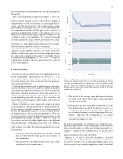
Figure 13 illustrates control input and output in a typical linear simulation. The linear system was initialized by scal- ing the (unique) unstable eigenvector to a displacement of 4.5 cm. The initial time was set to 1.4 ms to match the ini- tial displacement of the non-linear simulations. The con- trol system activates when the displacement reaches 5.2 cm and immediately assigns a voltage of ±800 V to each coil. The currents in the coils differ slightly due to the different mutual inductances with plasma and other coils. With in- spiration from the terminology used for analysis of second order systems, we define the following quantities (for stabi- lized systems):
• The offset is the average position after the settling time (as defined below) has passed, in the limit of a long simulation.
• The amplitude is the RMS deviation from the offset, calculated over the same period.
8 6 4 2 0 2
300 150 0 150 300 1600 800 0 800 1600
2 3 4 5 6 7 8 9 10 Time [ms]
FIG. 13. Separatrix location, control coil currents, and control coil voltages in a representative linear, closed-loop simulation. In this case, the cycle time was 25 μs, the latency one cycle, and the overall gain 25. (There are 8 different graphs for current and voltage that are mostly on top of each other; only the first 10 ms of a 30 ms simulation are plotted).
• The period is the average time that passes between crossings of the offset with negative slope, calculated over the same period.
• If the position is not eventually bounded by ±5.2 cm (the displacement at which feedback activates), the settling time is not defined and the above quantities are calculated starting from the beginning of the sim- ulation. Otherwise the settling time is the earliest time at which the position returns to offset without af- terwards exceeding ±5.2 cm.
For a given simulation, we calculate these values by start- ing with a high estimate of the settling time (3 ms) and then iterate the calculation of offset and settling time until con- vergence. In figure 13, the settling time is 3.1 ms, the offset is 0.05 cm, the amplitude is 0.4 cm, and the period is 452 μs. Linear simulations were run until 30 ms.
Figures 14, 15 and 16 show the dependence of period and amplitude on feedback gain, cycle time, and latency. The general trends are not surprising. Higher gain results in faster periods and smaller amplitudes until a threshold
Voltage [V]
Current [A]
Position [cm]