Page 9 - Positional stability of field-reversed-configurations in the presence of resistive walls

9
140 120 100
80 60 40 20
0
0 10 20 30 40 50
Displacement [cm]
Act
ual Value
Linear Prediction
cyl_60cm_120cm
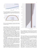
FIG. 8. Linearized driving force versus actual driving force for in- creasing plasma displacement. This plot indicates that mathemat- ically a linear approximation might be valid for displacements up to about 20 cm.
0.157 cm
FIG. 9. Re-centered separatrix traces over time (run with nominal wall conductivity). For a rigidly displaced plasma, the traces would be perfectly overlaid.
and calculating ⃗jp × B⃗v). The plasma current and vacuum fields were taken from t = 1 ms, but are expected to vary lit- tle over time. The rigid volume was taken as a spheroid with minor radius 47 cm and major radius 92 cm. Based on this plot we would expect that the linear approximation might be valid for displacements up to about 20 cm.
Figure 9 provides a measure of the “rigidity” of the in- stability. It has been generated by taking snapshots of the separatrix over time, re-centering each snapshot (by sub- tracting the center location from each coordinate), and then overplotting all the snapshots, labelled by the displacement. For a perfectly rigid displacement, these snapshots would all coincide exactly. The deviations are sufficiently small to make it plausible that the instability may be approximated as being rigid.
The simplest verifiable prediction of the linear model is the dependence of the growth time on wall resistivity. From equation (29) we can see that if the wall resistivity is scaled, the eigenvalues of the system are scaled by the same factor. From table I we can see that this is reproduced in the non- linear simulation rather well. For example, scaling the wall conductivity to 50% of its nominal value results in an insta- bility growth time that’s 50.6% as fast.
Another prediction of the linear model is that growth rates will be independent of plasma mass and temperature. For example, multiplying the plasma density by two and di- viding the temperature by the same value (to preserve force balance) does not change the predicted stability properties.
cyl_54cm_108cm spheroid_60cm_120cm spheroid_54cm_108cm cyl_60cm_90cm spheroid_60cm_90cm cyl_54cm_81cm spheroid_54cm_81cm spheroid_50cm_100cm cyl_48cm_96cm spheroid_48cm_96cm cyl_48cm_72cm cyl_46cm_92cm spheroid_48cm_72cm spheroid_46cm_92cm cyl_44cm_88cm spheroid_44cm_88cm cyl_42cm_84cm spheroid_42cm_84cm cyl_40cm_80cm spheroid_40cm_80cm
1 ms 2 ms 3 ms
600 700
40 35 30 25 20 15 10
5 0
z= z= z=
z=
z=
0.010 cm 0.044 cm 0.083 cm
0.116 cm
80 60 40 20 0 20 40 60 80 Z [cm]
0
100 200 300
Time Constant [ s]
FIG. 10. Instability growth times predicted by the linear model for different rigid volumes. Colors indicate the time at which the plasma has been linearized. Vertical lines indicate the values ob- tained by least-squares fitting of the non-linear simulations (with 10% uncertainty).
However, this prediction can not be tested with the Q2D code: while we can change the initial plasma density and plasma temperature, this change results in a very different plasma when transport and fast particle effects are taking effect during the settling period.
The most important prediction of the linear model is thus the growth times of the instability. The prediction for the growth time, however, depends on the choice of rigid volume, so comparing it with the non-linear results is non-trivial. Figure 10 shows an overview of the differ- ent growth times that are predicted by the linear model for different choices of rigid volumes. Two kinds of rigid vol- umes were used: a set of cylinders with different radii and half-lengths (“cyl”), and a set of spheroids with different radii (“spheroid”). The variation is considerable, so that in principle one could obtain a prediction of any arbitrary
400 500
R [cm] Driving Force [N]