Page 2 - Calibration and applications of visible imaging cameras on the C-2U advanced beam-driven field-reversed configuration device

10E103-2 Granstedt, Fallah, and Thompson
Rev. Sci. Instrum. 89, 10E103 (2018)
FIG. 1. Viewing geometry and machine coordinate system for the (a) axial and (b) radial cameras. The axial and radial viewport locations are (x, y, z) = (0, −0.68, 2.1) and (0.67, 0.19, 0.48) m, respectively. The ellipsoid represents an FRC with radius 0.35 m and elongation 3.0. Note that the DC magnetic field is along +z. Reproduced with permission from Granstedt et al., Rev. Sci. Instrum. 87, 11D416 (2016). Copyright 2016 AIP Publishing LLC.
if the optical system were perfectly rigid, only the external calibration would need to be determined in situ.
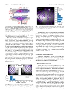
The camera spatial calibration was determined ex situ to provide an initial estimate for the in situ calibration. First, images were recorded of a checkerboard pattern of 3.0 cm squares in various orientations and distances relative to the camera optics. Note that it is essential that the image sequence contains the checkerboard pattern at various angles relative to the optics; otherwise, magnification and distance parameters cannot be distinguished. Second, the pixel locations of the inte- rior checkerboard corners were determined using an algorithm from OpenCV.7 For each image, the positions of the corners are known in physical space, relative to a global translation and rotation; therefore, the full set of unknown parameters consists of six external calibration coefficients for each image, along with the radially symmetric, distortion, and internal calibra- tion coefficients of the camera model. Finally, these parameters were determined using a non-linear least-squares optimization algorithm. Sample results from typical calibration images are displayed in Fig. 2.
FIG. 2. Radial camera ex situ spatial calibration: (a) Sample images of the checkerboard target with corner positions extracted from images (“datums”) and re-mapped locations using camera model (“mapping”). (b) Histogram of residual errors.
FIG. 3. Radial camera in situ spatial calibration: (a) Dα image of the vessel interior, with manually positioned port outlines in blue and projected outlines in magenta. (b) Histogram of residual errors.
After installation on C-2U, camera spatial calibration was performed in situ. Images were selected from shots where plasma-related emission provided good illumination of the interior of the vacuum vessel (e.g., Dα images immediately after FRC formation). Next, the vessel CAD geometry was used to compute port outlines in the inner vacuum vessel wall. The estimated camera orientation and position were used with the ex situ spatial calibration to project these port outlines onto the camera images. These projected camera images were then manually re-aligned to match the port outlines visible in the images. Finally, the spatial calibration parameters were numer- ically optimized to get the best match between the mapped port outlines (“mapping” in Fig. 3) and the manually adjusted contours (“datums” in Fig. 3).
III. RADIOMETRIC CALIBRATION
Radiometric calibration of the full optical system com- prised three stages: finding the camera relative response func- tion, the optical system non-uniformity, and the absolute photon sensitivity using each interference filter.
A. Camera relative response
Intrinsic physical processes in the CMOS sensors used in high-speed cameras introduce non-linearity in the detector response to photon illumination.8 In addition, camera manu- facturers often incorporate nonlinear digital processing (e.g., gamma correction) to form a more attractive image. Although linear response is generally considered preferable for scientific instruments, non-linearity in the form of reduced response near saturation has the benefit of increasing the overall dynamic range of the sensor. In fact, many sensors used in high-speed cameras incorporate the capability to intentionally add non- linearity specifically for this purpose. This feature is known as a “dual-slope shutter”9 or “extended dynamic range”10 (EDR). At one or more times during the integration, pixel voltages exceeding a threshold are reset to the threshold value. The result is that pixels near saturation exhibit reduced photon response while those far from saturation are unaffected. Images of plasma light emission often contain regions with vastly