Page 3 - Calibration and applications of visible imaging cameras on the C-2U advanced beam-driven field-reversed configuration device

10E103-3 Granstedt, Fallah, and Thompson
different brightness: precisely the situation where the extended dynamic range is useful; nevertheless, this feature is rarely used because it is not understood or because of calibration challenges.
The relative response calibration maps detector counts to a linearized relative radiance that accounts for camera settings: integration time, extended dynamic range, and gain factors. The approach in this work adopts an algorithm from “High Dynamic Range” imaging:11 many images of a static scene are recorded using different camera settings. Since the scene is static, the radiance for each image is equal. Starting with an initial linear response, the response function and scene radi- ance are solved iteratively until convergence. Note that the relative response of each pixel is assumed to be identical within a scale factor and the illumination on the sensor does not need to be uniform. Non-uniformity correction of gains and offsets of individual pixels is left to the camera manufacturer.
The relative response function, Ne(C), was parameterized as an N-th-order polynomial with an additional stepwise linear function,9 Npe(Ne), if EDR was used,
N−1
Ne(C)=􏰄ckCk, (1a)
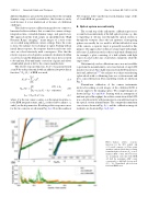
Rev. Sci. Instrum. 89, 10E103 (2018) SC1 response (blue) and the increased dynamic range of the
v5.2 with EDR on (green).
B. Optical system non-uniformity
The second step of the radiometric calibration process to account for non-uniformity of the full optical system, e.g., due to vignetting of off-axis rays through the optical system or through the viewport. Since the exit apertures of integrating spheres are usually far too small to fill the full field-of-view of the camera, a separate target is generally needed for this purpose. One approach is to fabricate a large target with a high- reflectance Lambertian surface that is uniformly illuminated; for example, a plate consisting of a half-cylinder with light sources located on the axis of curvature, symmetric about the target center.3
Unfortunately, such a calibration source was not available to perform the nonuniformity correction. Instead, a large LCD monitor was used. Since light emission from LCD monitors is far from Lambertian,12,13 the radiance was characterized using a photodiode with a collimating lens on a rotation mount and fit to a smooth function. Data and fitting results are shown in Fig. 5.
Nonuniform calibration of the camera instruments involved recording several images of the calibrated LCD at various angles to the imaging optics. Two sample images are shown in Figs. 6(a) and 6(b). Starting with an assumption of uniform optical throughput, the relative orientation of the LCD was solved iteratively with parameters in a model function for the optical system nonuniformity. The computed nonuniform correction is shown in Fig. 6(c), and the calibration image fit residuals are shown in Figs. 6(d)–6(f).
Ne Npe(Ne) = 
, (1b) (1c)
k=0
if Ne ≤ d0 d0 + t0/t1(Ne − d0) otherwise

Lrel = Npe(Ne(C))/t0,
where C is the raw camera counts, t0 is the integration time, t1 is the EDR integration time, and Lrel is the relative radiance. ck and d0 are the fit parameters. Resulting relative response curves for the two cameras are shown in Fig. 4(a). Note the nonlinear
FIG.4. Camera relative response functions for the SC1 (radial) and v5.2 (axial) cameras. (a) Data points (markers) and fits (black lines) relating normalized photoelectrons (N pe ) to nor- malized ADC counts. Photoelectrons are normalized such that with EDR off, half the maximum ADC counts correspond to a half-full electron well (N w ). (b) Normalized photoelectron fractional RMS error.