Page 11 - Demo

042504-11 Rath et al.
Phys. Plasmas 24, 042504 (2017)
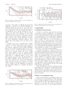
FIG. 14. Comparison of linear and non-linear closed loop simulations near the predicted optimum cycle time of 30 ls.
cycle time of 30ls. Here, we find that the linear model significantly overestimates the saturated amplitudes and oscillation periods for cycle times of 35ls and above. For cycle times below this value, the agreement is satis- factory. This indicates that the predictions from Figure 9 are qualitatively correct, but the dependency is not as strong as the linear model indicates. The most likely explanation for this is the representation of the control coils: in the linear model, they are represented as thin fil- aments, while in the non-linear simulation, they have finite extent and volume currents. This leads to a differ- ence in the self-inductance and thus a difference in the currents that becomes bigger as the cycle time becomes bigger.
Looking at the effects of varying latencies (Figures 15 and 16), we find good agreement for most cases. For a latency of 7 cycles, linear and non-linear simulations agree with the oscillation period and oscillation amplitude. However, the non-linear simulation makes a steep excur- sion from 6cm to þ12cm near 4ms that is superim- posed on the oscillatory behavior. We do not consider this a critical difference because the simulation quickly settles down to the same offset as in the linear code again. However, a significant difference can be found with a latency of 6 cycles. Here, the linear prediction of the saturated amplitude is much smaller than the non- linear value at all times. The reason for this discrepancy is not clear, and it seems to be specific to this latency (while not plotted, the agreement for latencies of 8 and 9 cycles is equally good) and equilibrium (in simulations with other initial conditions, no comparable discrepancies were found).
FIG. 16. Comparison of linear and non-linear closed loop simulations near the predicted maximum latency of 13 cycles (130 ls).
VI. DISCUSSION
A. Suitability of the linear model
Overall, we consider the agreement between the linear and non-linear closed loop simulations to be sufficiently good for control algorithm design. The linear model reprodu- ces the global behavior of the controlled system (amplitudes, periods, and return times) over a wide range of parameters and scale lengths. While there are some discrepancies for longer cycle times, it is expected that these can be fixed by using a more accurate representation of the control coils in the linear model. Comparisons were done over a period of 6 ms, which is much larger than all the relevant plasma time- scales (and in particular, the instability growth time), and so longer simulations are unlikely to reveal additional phenom- ena relevant to control of the positional instability.
Generally, the predictions of the linear model tend to overestimate the instability drive, which increases the confi- dence that algorithms designed for the linear model will also stabilize the non-linear system. However, we also found a single, so-far unexplained failure of the linear model for a specific, insulated set of parameters (gain 25, cycle time 10 ls, latency 6 cycles, cf. Figure 15). In this case, the linear model underestimates the saturated oscillation amplitude by about 50%. This emphasizes the need to eventually test every algorithm in a non-linear simulation but appears to be sufficiently rare to justify doing the majority of the design work using linear approximation.
The good performance of the linear model also provides further support for the assumption of a rigid displacement. If significant amounts of energy were stored or freed by defor- mations, the linear (rigid) model would be unlikely to repro- duce the behavior of the system over the range of parameters that we investigated.
B. Effects of non-axisymmetric walls
When used for modeling of axial displacements, the lin- ear model has the obvious advantage of being significantly faster to calculate. In addition to that, however, it also allows to incorporate the effects of a three dimensional wall—some- thing that is not possible when using an axisymmetric, non-linear code. The effects of a more realistic wall can be
FIG. 15. Comparison of linear and non-linear closed loop simulations near the predicted optimum latency of 6 cycles (60 ms).