Page 10 - Demo

042504-10 Rath et al.
Phys. Plasmas 24, 042504 (2017)
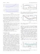
FIG. 10. Period and amplitude for different latencies in linear, closed-loop simulations. The gain was fixed at 25, and the cycle time was fixed at 10 ls.
sum. However, in the context of this work, we are not inter- ested in optimizing the algorithm but in the quality of the plant model, and so no such optimizations were attempted.
The linear model is expected to be valid for displace- ments up to 20cm. From the results of the scan, we can therefore make the following predictions for the non-linear behavior of the system:
• The minimum gain (with 10ls cycle time and 1 cycle latency) to stabilize the system is about 7 (lower gains result in oscillation amplitudes of more than 20 cm).
• The maximum cycle time (with gain 25 and one cycle latency) is about 60 ls.
• The maximum latency (with gain 25 and cycle time 10 ls) is 13 cycles, i.e., 130 ls.
• The optimum gain is about 30 (higher gains do not signifi- cantly decrease the oscillation amplitude or period).
• The optimum cycle time is about 30 ls.
• The optimum latency is about 6 cycles or 60 ls.
C. Non-linear results
Ideally, it would have been possible to include the results from non-linear simulations as a second series of datapoints in Figures 8–10. Unfortunately, this was not feasi- ble because the limited simulation time (not CPU time) available for non-linear simulations did not allow the deriva- tion of unique values for most of the plotted quantities. This can be readily seen from, e.g., Figure 7: had the simulation been terminated at 6ms (instead of extending until 30ms), we would have obtained a quite different (and incorrect) value for the offset (and thus also a much larger amplitude). In principle, we could have continued the non-linear simula- tion until after 6 ms, but in this case, the (slow but steady) changes in the unperturbed equilibrium would have made a comparison with the linear predictions pointless.
Instead, we therefore look at individual simulations with parameters close to the thresholds predicted by the linear model. When looking at these plots, it is important to keep in mind that each simulation runs independently in its own closed loop with a non-linear feedback algorithm, and so minuscule changes in the plasma state can cause huge differ- ences in the applied voltage. Therefore, corresponding
FIG. 12. Comparison of linear and non-linear closed loop simulations near the predicted optimum gain of 30.
simulations are not expected to result in matching graphs; rather, they should replicate the predictions of stability boundaries and global characteristics like oscillation periods and amplitudes.
Figure 11 compares the results of linear and non-linear simulations near the lower gain threshold of 7. The oscilla- tion period and amplitude agree. However, there are insuffi- cient data to determine if the non-linear simulations will go unstable or settle into a stable, large-amplitude oscillation.
If we look at the results near the predicted optimum gain of 30 (Figure 12), we find a similar situation. The initial evo- lution is predicted reasonably well, and arguably a gain of 40 does not improve upon a gain of 30, but the low number of (global) oscillations in the simulated time range makes it dif- ficult to make statements about saturated amplitudes or frequencies.
Figures 13 and 14 show results close to the predicted maximum stable cycle time of 60 ls and an optimum
FIG. 11. Comparison of linear and non-linear closed loop simulations near the predicted minimal gain of 7. (The near-perfect agreement with gain 10 is most likely due to chance and disappears again at gain 20.)
FIG. 13. Comparison of linear and non-linear closed loop simulations near the predicted maximum cycle time of 60 ls.